# === Cartesian Oval Lens for Optimal Fiber Coupling ===
#
# The Cartesian oval eliminates spherical aberration by enforcing a constant
# optical path length (OPL) for every ray from the point emitter to the
# collimated output plane.  For coupling into a single-mode fiber whose
# Gaussian mode has a flat wavefront at the fiber face $z_R >> d_cf$, the
# optimal design collimates the emitter's spherical wave into a plane wave.
#
# OPL condition:   $n_sil$ * sqrt$ρ² + z²$ - $n_out$ * z = $n_sil - n_out$ * h
#
# Closed-form:     z(ρ) = $n_out·h + n_sil·√$h² - κρ²$$ / $n_sil + n_out$
#                  κ = $n_sil + n_out$ / $n_sil - n_out$
#
# Valid aperture:  ρ ≤ ρ_max = h / √κ   (limited by total internal reflection)

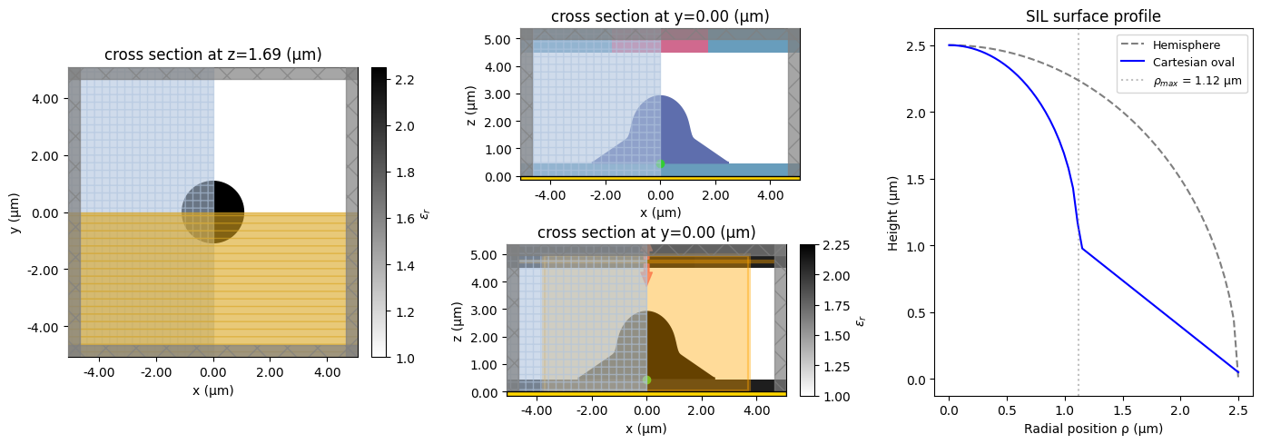
ring_radii = np.linspace$0.0, sil_radius, num_rings$
$h_apex$ = sil_radius  # On-axis apex height (matches hemisphere)

$n_out$ = 1.0  # Exit medium $air/vacuum$
kappa = $n_sil + n_out$ / $n_sil - n_out$
rho_max = $h_apex$ / np.sqrt(kappa)

# Cartesian oval profile within the TIR-limited aperture
discriminant = $h_apex$**2 - kappa * ring_radii**2
in_aperture = discriminant >= 0
oval_heights = np.where$in_aperture,
    ($n_out$ * $h_apex$ + $n_sil$ * np.sqrt(np.maximum(discriminant, 0)))
    / ($n_sil$ + $n_out$),
    0.0,$

# Beyond ρ_max: linear taper to min_height at the SIL edge
$h_edge$ = $n_out$ * $h_apex$ / $n_sil + n_out$  # Height at ρ = ρ_max
taper = $h_edge$ - $h_edge - min_height$ * $ring_radii - rho_max$ / $sil_radius - rho_max$
init_params = np.where$in_aperture, oval_heights, np.maximum(taper, min_height)$

theta_c = np.degrees$np.arcsin($n_out$ / $n_sil$)$
print$f"Cartesian oval:  κ = {kappa:.1f},  ρ_max = {rho_max:.3f} μm,  $h_edge$ = {$h_edge$:.3f} μm"$
print$f"Critical angle   = {theta_c:.1f}°"$

# Build and visualize simulation
init_sim = get_simulation$init_params$

fig = plt.figure$tight_layout=True, figsize=(14, 5)$
gs = fig.add_gridspec(2, 3)
ax1 = fig.add_subplot$gs[:, 0]$
ax2 = fig.add_subplot$gs[0, 1]$
ax3 = fig.add_subplot$gs[1, 1]$
ax4 = fig.add_subplot$gs[:, 2]$

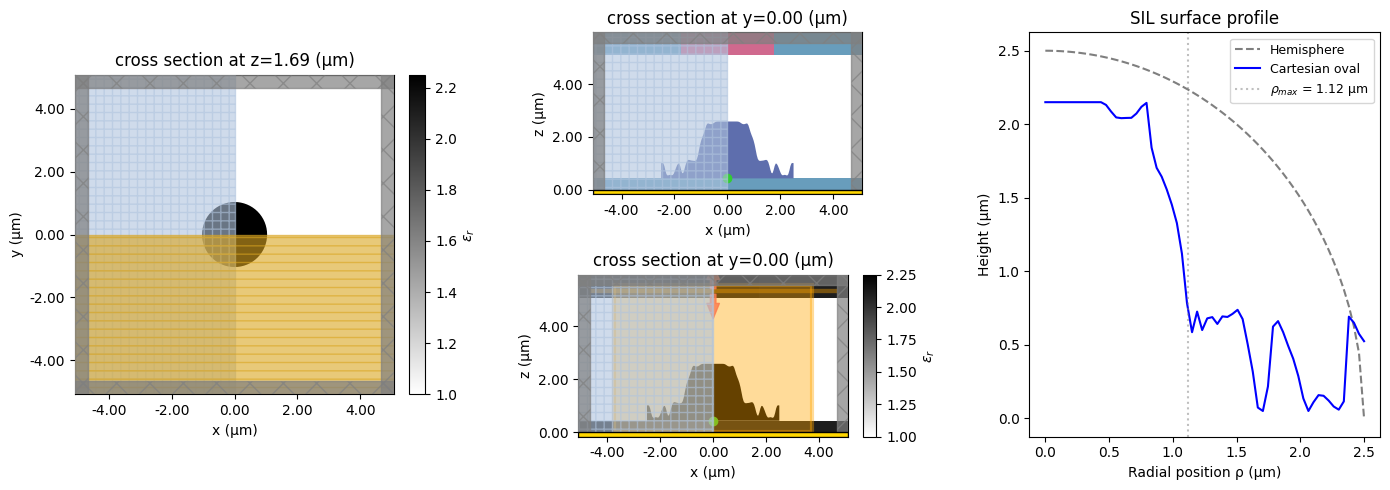
init_sim.plot_eps$z=$t_sio2$ + sil_radius / 2, ax=ax1, monitor_alpha=0$
init_sim.plot$y=0, ax=ax2, monitor_alpha=0$
init_sim.plot_eps$y=0, ax=ax3$

# Compare lens profiles
hemisphere = np.sqrt$np.maximum(sil_radius**2 - ring_radii**2, 0.0)$
ax4.plot$ring_radii, hemisphere, "k--", alpha=0.5, label="Hemisphere"$
ax4.plot$ring_radii, init_params, "b-", label="Cartesian oval"$
ax4.axvline$rho_max, color="gray", ls=":", alpha=0.5, label=f"$\\rho_{{max}}$ = {rho_max:.2f} μm"$
ax4.set_xlabel("Radial position ρ (μm)")
ax4.set_ylabel$"Height (μm)"$
ax4.set_title("SIL surface profile")
ax4.legend$fontsize=9$
plt.show()
Run 2026-03-24
init_params = np.array([2.15      , 2.15      , 2.15      , 2.15      , 2.15      ,
       2.15      , 2.15      , 2.15      , 2.15      , 2.15      ,
       2.15      , 2.15      , 2.1313322 , 2.086171  , 2.0464349 ,
       2.041331  , 2.0427978 , 2.0436196 , 2.0728662 , 2.1186922 ,
       2.1452532 , 1.8408425 , 1.7036216 , 1.6433294 , 1.55631   ,
       1.4533588 , 1.3277657 , 1.1201562 , 0.78409135, 0.58579063,
       0.72580475, 0.6003881 , 0.6798209 , 0.6882752 , 0.64195395,
       0.69327646, 0.6895122 , 0.7104395 , 0.7380386 , 0.6748007 ,
       0.50348157, 0.31806147, 0.07350177, 0.05      , 0.21639279,
       0.6237649 , 0.66108406, 0.58662486, 0.49266502, 0.4052913 ,
       0.28797153, 0.13498408, 0.05      , 0.10974871, 0.1578338 ,
       0.15337527, 0.12088381, 0.08042433, 0.05902958, 0.1153025 ,
       0.6914359 , 0.65003127, 0.57438517, 0.52466124], dtype=float32)

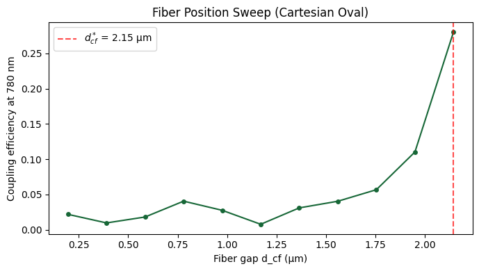
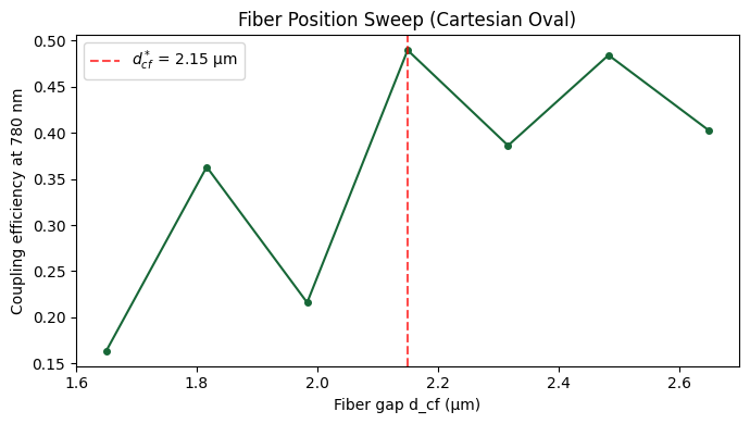
d_cf = 2.15
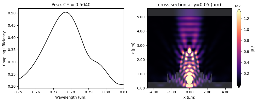
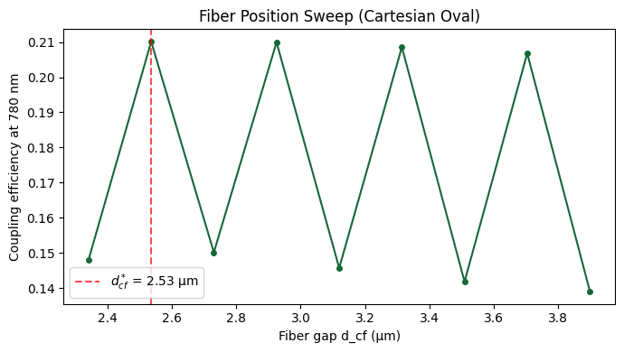
Doing a position sweep again
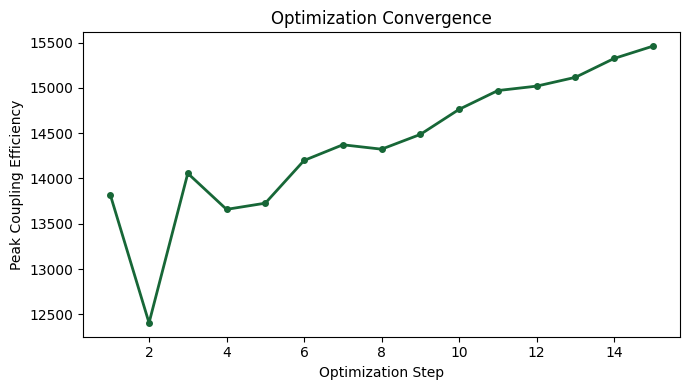
Updated params
array([2.15      , 2.15      , 2.15      , 2.15      , 2.15      ,
       2.15      , 2.15      , 2.15      , 2.15      , 2.15      ,
       2.15      , 2.15      , 2.097241  , 2.0641246 , 2.0564694 ,
       2.0771244 , 2.0746922 , 2.0511847 , 2.0654542 , 2.1104598 ,
       2.0746374 , 1.6593317 , 1.61374   , 1.7730736 , 1.6936587 ,
       1.5123912 , 1.3318948 , 1.0490649 , 0.6102792 , 0.42934996,
       0.7591557 , 0.75087565, 0.9297884 , 0.8957742 , 0.8042245 ,
       0.8338097 , 0.7845124 , 0.5903704 , 0.40914237, 0.27681845,
       0.35202086, 0.37775597, 0.3396622 , 0.36298108, 0.18884102,
       0.27224046, 0.4062518 , 0.62768054, 0.7888396 , 0.61301583,
       0.348251  , 0.05      , 0.05      , 0.05      , 0.05      ,
       0.13144836, 0.15863298, 0.05      , 0.29891923, 0.5672724 ,
       1.0776697 , 0.6546207 , 0.2848655 , 0.14540468], dtype=float32)
 \
\
[!ERROR] I realized that I was clipping the height of the lens. I am starting over with different constraints.
array([2.6623397 , 2.6353512 , 2.5762963 , 2.5094512 , 2.4548113 ,
       2.417729  , 2.3731413 , 2.288861  , 2.3609178 , 2.4291139 ,
       2.4739783 , 2.3005333 , 2.4113936 , 2.5722444 , 2.66333   ,
       1.8571405 , 1.9002906 , 1.9994804 , 2.0997105 , 2.121043  ,
       1.992148  , 1.8380157 , 1.9888959 , 2.331807  , 2.436948  ,
       1.4891073 , 1.1165357 , 1.1380515 , 1.4260321 , 1.5764182 ,
       1.3656145 , 0.6193609 , 0.3750911 , 0.5133566 , 0.7549467 ,
       0.9513143 , 1.0200113 , 0.77997386, 0.3790514 , 0.458539  ,
       0.58106464, 0.54539514, 0.32169437, 0.09893914, 0.1696058 ,
       0.35921615, 0.39739528, 0.36803186, 0.4783354 , 0.62903315,
       0.6235232 , 0.22600067, 0.05      , 0.05      , 0.05      ,
       0.15269797, 0.24259725, 0.17233059, 0.05139003, 0.05      ,
       0.05      , 0.5704556 , 0.7359599 , 0.7268702 ], dtype=float32)
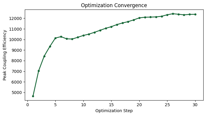
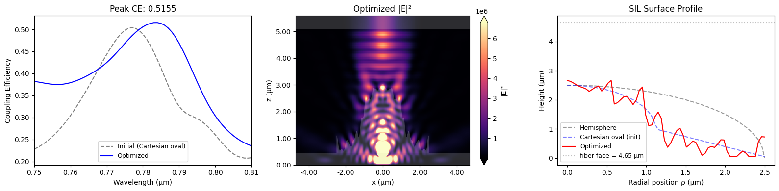
Optimizing again with no gold reflector
Optimization conditions - No backreflector - Azimuthal symmetry
First completed design
params = np.array([2.3806891  2.446803   2.5148678  2.4354632  2.2483227  2.4718928
 2.620887   2.5574138  2.5727844  2.9399548  2.9790215  2.7284467
 2.5522861  2.8535383  2.8400538  2.3388877  2.2373493  2.3052921
 2.3545012  2.108885   2.3334634  1.9900931  1.6770164  1.8462439
 1.930206   2.1130807  3.1932764  4.028008   1.1316414  0.05
 0.05       0.05       0.72253263 0.67029333 0.5386423  0.5216792
 0.52670884 0.6419068  0.5375593  0.5078126  0.7120204  1.2719915
 0.8124067  0.05       0.05       0.15194799 0.7220474  0.3473141
 0.12052727 0.41661236 1.0029374  0.32026052 0.05       0.05
 0.1289356  0.36760283 0.0958149  0.05       0.0500295  0.730262
 0.05       0.05       0.05       0.05      ])
Optimizing again to make sure
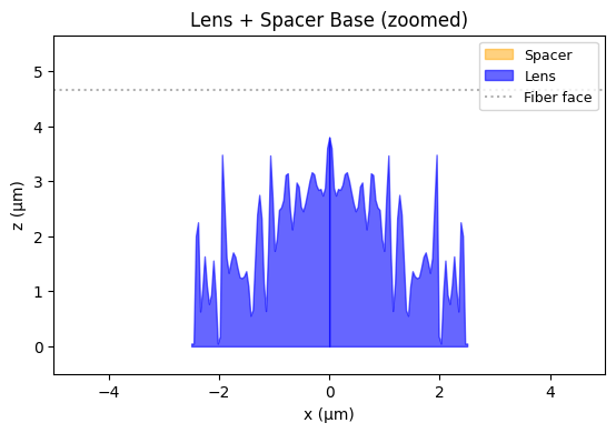
With this one, I started with a dome and optimized from there, instead of optimizing from a Cartesian oval.
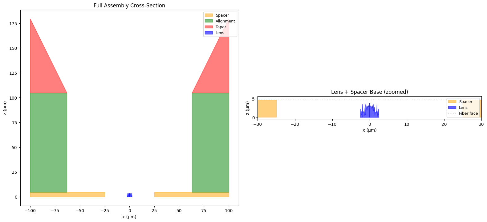
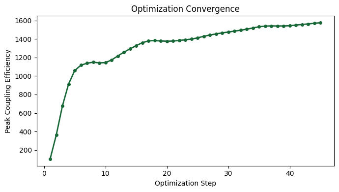
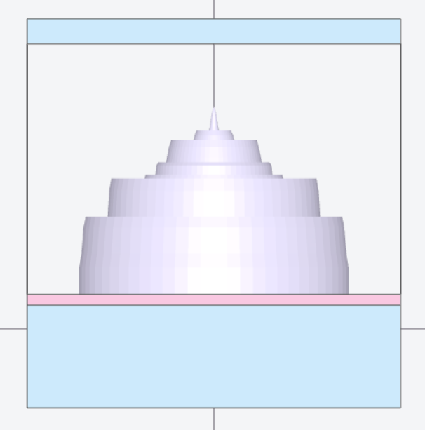
Just a simple Cartesian oval
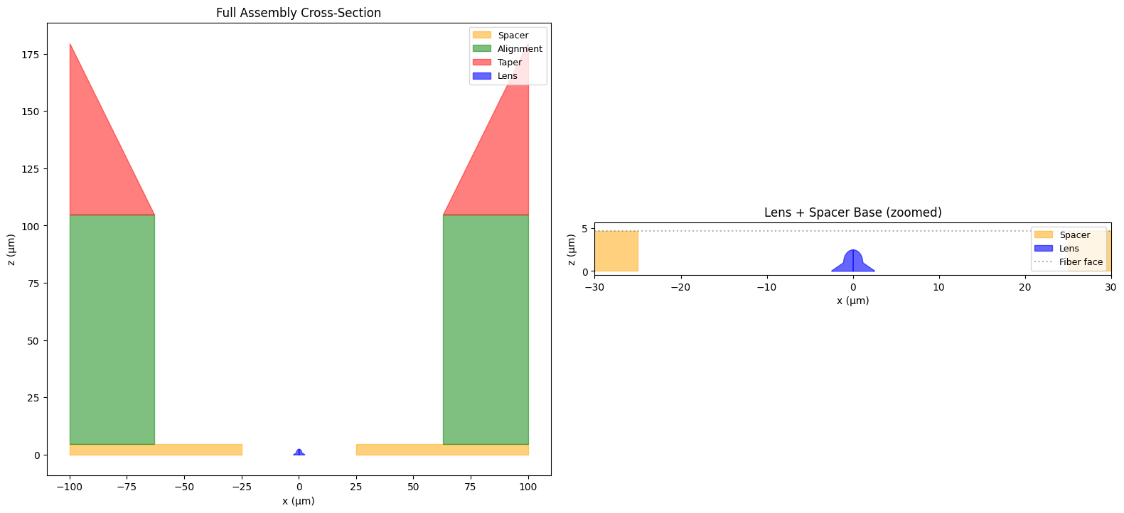
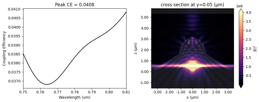
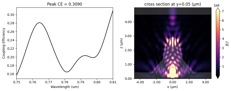
This design should still give a few million photons per second at 780 nm.