Inverse design of a high-Q nanobeam cavity

This executable tutorial starts from the validated nanobeam cavity, differentiates a fitted ringdown \(Q\) through a GPU-native FDTD solve, and validates the optimized design with a fresh long simulation of literal air cylinders. It follows the same practical structure as a Tidy3D inverse-design notebook: parameters, geometry, plotted material, differentiable simulation, optimization, final fields, and quantitative analysis.

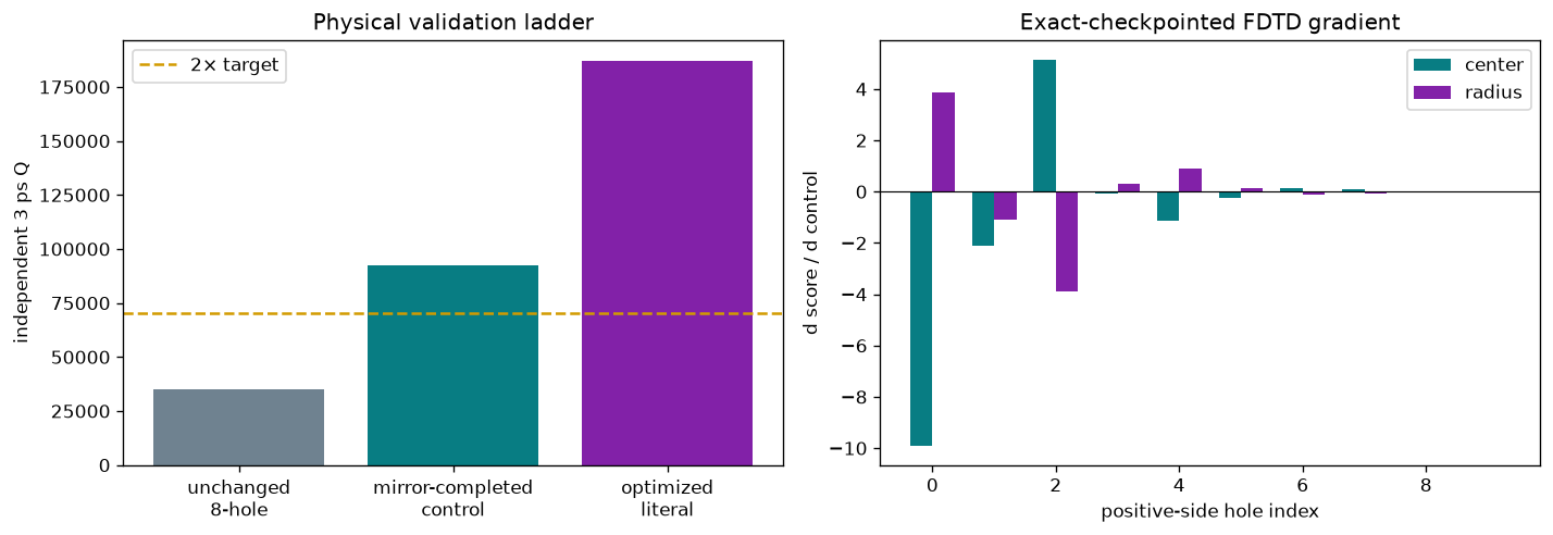
The acceptance test is deliberately harder than “the objective increased.” The final binary geometry must exceed twice the unchanged eight-hole cavity and must also beat an unoptimized, automatically mirror-completed control. The saved run uses one exact-checkpointed adjoint update from a zero-vector cold start—no optimized warm start, imported pixels, or Tidy3D solve is involved.

Imports and accelerator

import gc
import json
import os
os.environ.setdefault("XLA_PYTHON_CLIENT_PREALLOCATE", "false")

from pathlib import Path
from time import perf_counter
import warnings
import jax
import jax.numpy as jnp
import matplotlib.pyplot as plt
from matplotlib.patches import Circle, Rectangle
import numpy as np
import pandas as pd
from scipy.signal import hilbert
import fdtdx
from IPython import get_ipython

from benchmarks.cases.device_nanobeam_cavity.run import (
    NanobeamParameters,
    _dominant_resonance,
    build_nanobeam_simulation,
    run_nanobeam_simulation,
)
from benchmarks.cases.invdes_nanobeam_cavity.run import (
    ARTIFACT,
    BASELINE_Q,
    GUARANTEED_MIN_GAP_NM,
    MIRROR_COMPLETED_CONTROL_Q,
    NUM_DESIGN_HOLES,
    SAMPLES_PER_WINDOW,
    TARGET_Q,
    fabrication_metrics,
    optimize_nanobeam,
    physical_hole_geometry,
)
from benchmarks.device_geometry import nanobeam_holes_um

get_ipython().run_line_magic("matplotlib", "inline")
warnings.filterwarnings("ignore", category=FutureWarning, module=r"tidy3d\.components\.mode")
plt.rcParams.update({"figure.figsize": (10, 4.8), "figure.dpi": 120})
tidy_validation_path = ARTIFACT.parents[1] / "goldens" / "tidy3d_validation_invdes_nanobeam_cavity.npz"
print(f"JAX devices: {jax.devices()}")
print(f"Optimization artifact: {ARTIFACT.relative_to(ARTIFACT.parents[2])}")
print(f"Independent Tidy3D validation: {tidy_validation_path}")

JAX devices: [CudaDevice(id=0)]
Optimization artifact: benchmarks/artifacts/invdes_nanobeam_cavity_best.npz
Independent Tidy3D validation: /home/hoodlab/github/fdtdx-hoodlab/benchmarks/goldens/tidy3d_validation_invdes_nanobeam_cavity.npz

1. Physical, numerical, and optimization parameters

The forward benchmark uses a 25 nm Yee grid, 12 PML cells, x/y parity, a broadband \(E_y\) dipole, and a 3 ps validation ringdown. The differentiable solve uses only 0.8 ps: the source transient is discarded and three coherent 2,000-sample windows estimate one complex pole. Exact checkpointing trades compute for memory so the reverse pass fits on a 12 GB RTX 3080.

parameters = NanobeamParameters(
    grid_spacing_um=0.025,
    run_time_ps=3.0,
    analysis_start_ps=0.2,
    wavelength_window_um=(1.4, 1.6),
    beam_width_um=0.500,
    beam_thickness_um=0.220,
    pml_layers=12,
)
pd.Series({
    **parameters._asdict(),
    "positive-side shape controls": 2 * NUM_DESIGN_HOLES,
    "short-fit windows": 3,
    "samples per fit window": SAMPLES_PER_WINDOW,
    "unchanged baseline Q": BASELINE_Q,
    "required Q (2× baseline)": TARGET_Q,
    "mirror-completed control Q": MIRROR_COMPLETED_CONTROL_Q,
    "guaranteed minimum bridge (nm)": GUARANTEED_MIN_GAP_NM,
}, name="value").to_frame()

	value
grid_spacing_um	0.025
interior_um	(8.4, 3.7, 3.4)
run_time_ps	3.0
analysis_start_ps	0.2
wavelength_window_um	(1.4, 1.6)
pml_layers	12
beam_width_um	0.5
beam_thickness_um	0.22
silicon_index	3.5
oxide_index	1.44
positive-side shape controls	20
short-fit windows	3
samples per fit window	2000
unchanged baseline Q	35125.300715
required Q (2× baseline)	70250.60143
mirror-completed control Q	92493.301338
guaranteed minimum bridge (nm)	65.0

2. Initial geometry and automatic mirror completion

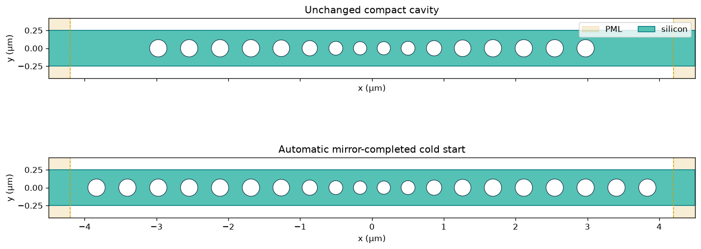
The original compact example has eight positive-side holes. High-Q optimization is otherwise capped by leakage through that short mirror, so extend_periodic_mirror_to_boundary appends complete nominal periods while the hole edge remains inside the non-PML domain. The silicon beam already crosses the PML. The helper adds two holes per side here; it does not tune the cavity taper.

original_centers_um, original_radii_um = nanobeam_holes_um()
zero_controls = np.zeros(2 * NUM_DESIGN_HOLES, dtype=np.float32)
control_centers_um, control_radii_um = physical_hole_geometry(zero_controls)

def draw_geometry(ax, centers, radii, title):
    domain_half = parameters.interior_um[0] / 2 + parameters.pml_layers * parameters.grid_spacing_um
    interior_half = parameters.interior_um[0] / 2
    ax.axvspan(-domain_half, -interior_half, color="#d9a21b", alpha=0.18, label="PML")
    ax.axvspan(interior_half, domain_half, color="#d9a21b", alpha=0.18)
    ax.add_patch(Rectangle(
        (-domain_half, -parameters.beam_width_um / 2),
        2 * domain_half, parameters.beam_width_um,
        facecolor="#55c2b5", edgecolor="#087d83", label="silicon",
    ))
    for center, radius in zip(centers, radii, strict=True):
        ax.add_patch(Circle((center, 0), radius, facecolor="white", edgecolor="#18364a", lw=0.7))
    ax.axvline(-interior_half, color="#d29b00", ls="--", lw=0.9)
    ax.axvline(interior_half, color="#d29b00", ls="--", lw=0.9)
    ax.set(xlim=(-domain_half, domain_half), ylim=(-0.42, 0.42), aspect="equal", title=title,
           xlabel="x (µm)", ylabel="y (µm)")

fig, axes = plt.subplots(2, 1, figsize=(12, 5.5), sharex=True)
draw_geometry(axes[0], original_centers_um, original_radii_um, "Unchanged compact cavity")
draw_geometry(axes[1], control_centers_um, control_radii_um, "Automatic mirror-completed cold start")
axes[0].legend(loc="upper right", ncol=2)
plt.tight_layout()
plt.show()

print(f"Full holes: {len(original_centers_um)} → {len(control_centers_um)}")
print(f"Last hole edge: {control_centers_um[-1] + control_radii_um[-1]:.3f} µm; non-PML edge: {parameters.interior_um[0]/2:.3f} µm")

Full holes: 16 → 20
Last hole edge: 3.955 µm; non-PML edge: 4.200 µm

3. Differentiable fitted-Q objective

Each short ringdown window is coherently demodulated near the tracked resonance. A complex ratio fit gives \(z=\exp[(-\gamma+i\Delta\omega)T]\), then \(Q=\pi f/\gamma\). Because this estimator is written entirely in JAX, its scalar Q can be reverse-differentiated through the complete time-domain solve.

The physical forward raster is not a grey sigmoid. It is the same binary 8×8 subcell fill fraction and diagonal Farjadpour interface tensor used by literal cylinders. A sigmoid boundary is used only for its straight-through shape derivative. Residual, window-consistency, amplitude, positive-decay, and wavelength guards prevent the optimizer from selecting a meaningless fitted pole.

# This call runs one cold-start adjoint when no compatible artifact exists.
# On an executed release notebook it resumes the saved passing stage and performs
# no additional speculative updates; the fresh validation solves below still run.
started = perf_counter()
optimization = optimize_nanobeam(iterations=1)
setup = optimization.pop("setup", None)
del setup
gc.collect()

artifact = np.load(ARTIFACT, allow_pickle=True)
best_controls = np.asarray(artifact["best_parameters"])
history = json.loads(str(artifact["history_json"]))
print(f"Accepted adjoint updates: {len(history)}")
print(f"Cold-start control norm: {np.linalg.norm(history[0]['parameters_before']):.1f}")
print(f"Notebook replay/setup time: {perf_counter() - started:.1f} s")
pd.DataFrame(history)[[
    "step", "quality_factor_before", "quality_factor", "fit_residual",
    "window_consistency", "gradient_norm", "accepted_trust_radius", "backtracks",
]]

Accepted adjoint updates: 1
Cold-start control norm: 0.0
Notebook replay/setup time: 18.0 s

	step	quality_factor_before	quality_factor	fit_residual	window_consistency	gradient_norm	accepted_trust_radius	backtracks
0	0	83600.84375	156639.46875	0.00021	0.154287	12.755676	0.075	1

4. Optimization history and the actual adjoint gradient

first = history[0]
gradient = np.asarray(first["gradient"])
indices = np.arange(NUM_DESIGN_HOLES)

fig, axes = plt.subplots(1, 2, figsize=(12, 4.2))
stages = ["unchanged\n8-hole", "mirror-completed\ncontrol", "optimized\nliteral"]
long_q = [BASELINE_Q, MIRROR_COMPLETED_CONTROL_Q, float(artifact["validated_q"])]
colors = ["#6f8290", "#087d83", "#8221a8"]
axes[0].bar(stages, long_q, color=colors)
axes[0].axhline(TARGET_Q, color="#d29b00", ls="--", label="2× target")
axes[0].set(ylabel="independent 3 ps Q", title="Physical validation ladder")
axes[0].legend()

axes[1].bar(indices - 0.18, gradient[:NUM_DESIGN_HOLES], width=0.36, label="center", color="#087d83")
axes[1].bar(indices + 0.18, gradient[NUM_DESIGN_HOLES:], width=0.36, label="radius", color="#8221a8")
axes[1].axhline(0, color="black", lw=0.7)
axes[1].set(xlabel="positive-side hole index", ylabel="d score / d control", title="Exact-checkpointed FDTD gradient")
axes[1].legend()
plt.tight_layout()
plt.show()

pd.Series({
    "short fitted Q before": first["quality_factor_before"],
    "short fitted Q after": first["quality_factor"],
    "accepted": first["accepted"],
    "line-search backtracks": first["backtracks"],
    "adjoint wall time (s)": first["elapsed_seconds"],
}, name="value").to_frame()

	value
short fitted Q before	83600.84375
short fitted Q after	156639.46875
accepted	True
line-search backtracks	1
adjoint wall time (s)	249.182671

5. Final binary geometry and voxelized material

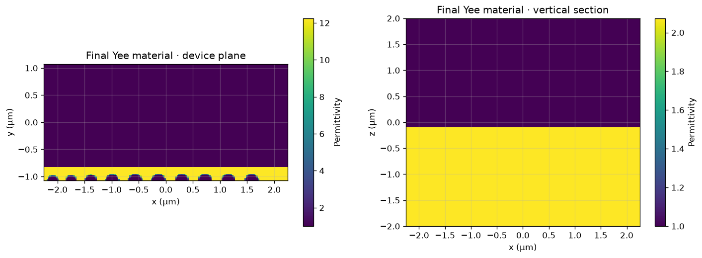
The unconstrained optimizer variables are mapped through bounded tanh transforms: centers can move by at most 25 nm and radii by at most 15 nm. Those hard bounds make the 65 nm minimum bridge a geometric guarantee, not a penalty that might be violated. The plotted circles below are the exact arrays passed to the final forward builder.

final_centers_um, final_radii_um = physical_hole_geometry(best_controls)
fabrication = fabrication_metrics(best_controls)

fig, ax = plt.subplots(figsize=(12, 2.9))
draw_geometry(ax, final_centers_um, final_radii_um, "Final optimized literal-cylinder geometry")
ax.legend(loc="upper right", ncol=2)
plt.tight_layout()
plt.show()

positive = slice(NUM_DESIGN_HOLES, None)
geometry_table = pd.DataFrame({
    "control x (µm)": control_centers_um[positive],
    "optimized x (µm)": final_centers_um[positive],
    "Δx (nm)": 1e3 * (final_centers_um[positive] - control_centers_um[positive]),
    "control r (µm)": control_radii_um[positive],
    "optimized r (µm)": final_radii_um[positive],
    "Δr (nm)": 1e3 * (final_radii_um[positive] - control_radii_um[positive]),
})
display(geometry_table.round(5))
pd.Series(fabrication, name="value").to_frame()

	control x (µm)	optimized x (µm)	Δx (nm)	control r (µm)	optimized r (µm)	Δr (nm)
0	0.16500	0.16355	-1.45445	0.09240	0.09274	0.34064
1	0.50281	0.50250	-0.31162	0.09677	0.09668	-0.09714
2	0.86562	0.86638	0.75556	0.10640	0.10606	-0.34333
3	1.26281	1.26280	-0.01012	0.11602	0.11605	0.02641
4	1.68500	1.68483	-0.16894	0.12040	0.12048	0.07917
5	2.11500	2.11496	-0.03729	0.12040	0.12041	0.01162
6	2.54500	2.54502	0.02160	0.12040	0.12039	-0.01062
7	2.97500	2.97502	0.01592	0.12040	0.12039	-0.00539
8	3.40500	3.40500	0.00364	0.12040	0.12040	-0.00024
9	3.83500	3.83500	-0.00182	0.12040	0.12040	0.00121

	value
minimum_silicon_gap_nm	141.609818
minimum_hole_diameter_nm	185.481277
fabrication_violation_nm	0.000000

object_list, constraints, config = build_nanobeam_simulation(
    parameters,
    hole_centers_um=final_centers_um,
    hole_radii_um=final_radii_um,
)
key = jax.random.PRNGKey(0)
objects, arrays, design_params, config, _ = fdtdx.place_objects(
    object_list=object_list, config=config, constraints=constraints, key=key,
)
arrays, objects, _ = fdtdx.apply_params(arrays, objects, design_params, key)

fig, axes = plt.subplots(1, 2, figsize=(12, 4.2))
fdtdx.plot_material_from_side(config, arrays, viewing_side="z", position=0.0,
                              material_axis=0, plot_legend=True, ax=axes[0])
fdtdx.plot_material_from_side(config, arrays, viewing_side="y", position=0.0,
                              material_axis=0, plot_legend=True, ax=axes[1])
axes[0].set_title("Final Yee material · device plane")
axes[1].set_title("Final Yee material · vertical section")
plt.tight_layout()
plt.show()
del arrays, objects, object_list
gc.collect()

13963

6. Fresh baseline and final FDTD simulations

These are not optimizer-surrogate plots. Both scenes are rebuilt from ordinary Cylinder objects and propagated for 3 ps. The baseline uses the unchanged default geometry; the final run uses the optimized center/radius arrays above. Terminal fields and complete point-monitor ringdowns are retained for the plots that follow.

started = perf_counter()
baseline_sim = run_nanobeam_simulation(parameters, record_field=True, show_progress=False)
baseline_seconds = perf_counter() - started
started = perf_counter()
final_sim = run_nanobeam_simulation(
    parameters, record_field=True, show_progress=False,
    hole_centers_um=final_centers_um, hole_radii_um=final_radii_um,
)
final_seconds = perf_counter() - started
print(f"Baseline GPU solve: {baseline_seconds:.1f} s")
print(f"Final GPU solve:    {final_seconds:.1f} s")
print(f"Reduced grid: {final_sim.objects.volume.grid_shape}; time steps: {final_sim.config.time_steps_total:,}")

Baseline GPU solve: 33.7 s
Final GPU solve:    33.2 s
Reduced grid: (180, 86, 160); time steps: 62,940

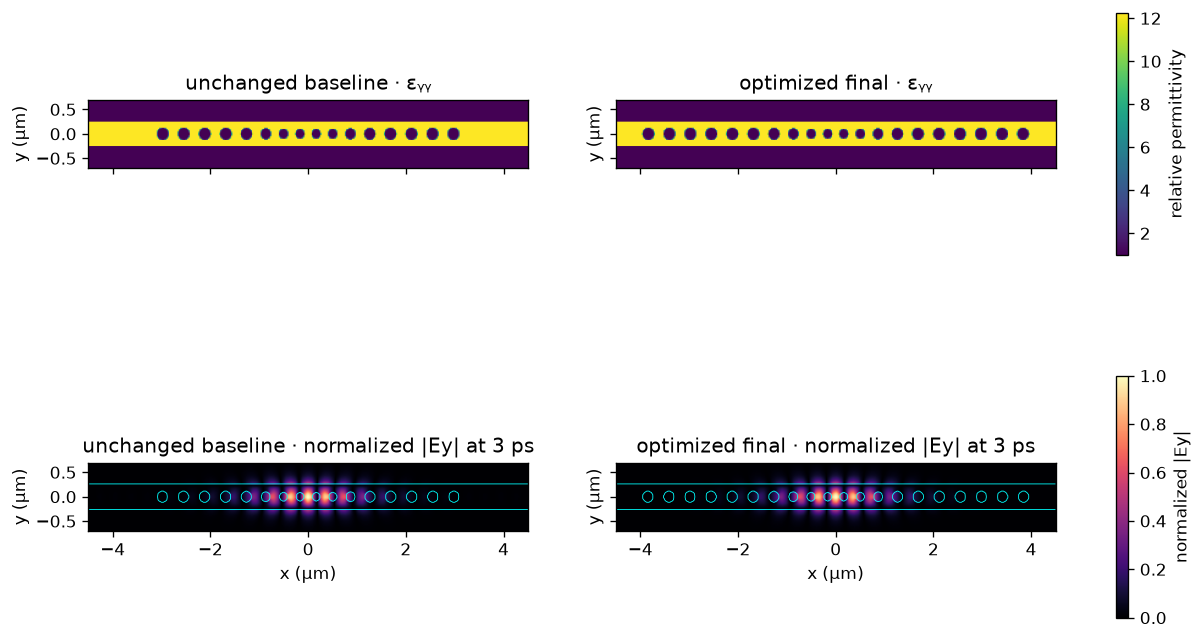
7. Material and electric-field profiles

def unfold_quarter(values):
    values = np.asarray(values)
    full_x = np.concatenate((values[::-1, :], values), axis=0)
    return np.concatenate((full_x[:, ::-1], full_x), axis=1)

domain_x = parameters.interior_um[0] / 2 + parameters.pml_layers * parameters.grid_spacing_um
domain_y = parameters.interior_um[1] / 2 + parameters.pml_layers * parameters.grid_spacing_um
extent = [-domain_x, domain_x, -domain_y, domain_y]

fig, axes = plt.subplots(2, 2, figsize=(13, 7.2), sharex=True, sharey=True)
for column, (label, sim) in enumerate((("unchanged baseline", baseline_sim), ("optimized final", final_sim))):
    eps = 1 / np.asarray(sim.arrays.inv_permittivities[1])
    eps_xy = unfold_quarter(eps[:, :, eps.shape[2] // 2])
    ey_xy = unfold_quarter(np.abs(sim.field_snapshot))
    material = axes[0, column].imshow(eps_xy.T, origin="lower", extent=extent, cmap="viridis", aspect="equal")
    field = axes[1, column].imshow(
        (ey_xy / (ey_xy.max() + 1e-30)).T, origin="lower", extent=extent,
        cmap="magma", vmin=0, vmax=1, aspect="equal",
    )
    axes[1, column].contour(
        np.linspace(extent[0], extent[1], eps_xy.shape[0]),
        np.linspace(extent[2], extent[3], eps_xy.shape[1]),
        eps_xy.T, levels=[2.0], colors="cyan", linewidths=0.5,
    )
    axes[0, column].set_title(f"{label} · εᵧᵧ")
    axes[1, column].set_title(f"{label} · normalized |Ey| at 3 ps")
for ax in axes.flat:
    ax.set(xlim=(-4.5, 4.5), ylim=(-0.7, 0.7), ylabel="y (µm)")
axes[1, 0].set_xlabel("x (µm)")
axes[1, 1].set_xlabel("x (µm)")
fig.colorbar(material, ax=axes[0, :], shrink=0.8, label="relative permittivity")
fig.colorbar(field, ax=axes[1, :], shrink=0.8, label="normalized |Ey|")
plt.show()

8. Ringdown, fitted pole, and spectrum

sample_dt = 2 * final_sim.config.time_step_duration
time_ps = parameters.analysis_start_ps + np.arange(final_sim.ringdown.size) * sample_dt * 1e12
baseline_pole = _dominant_resonance(baseline_sim.ringdown, sample_dt)
final_pole = _dominant_resonance(final_sim.ringdown, sample_dt)

fig, axes = plt.subplots(1, 3, figsize=(15, 4.2))
for signal, label, color in (
    (baseline_sim.ringdown, "baseline", "#087d83"),
    (final_sim.ringdown, "optimized", "#8221a8"),
):
    normalized = signal / np.max(np.abs(signal))
    axes[0].plot(time_ps[::4], normalized[::4], lw=0.65, label=label, color=color)
    envelope = np.abs(hilbert(signal))
    axes[1].semilogy(time_ps[::10], (envelope / envelope.max())[::10], lw=1.0, label=label, color=color)

    frequencies = np.fft.rfftfreq(signal.size, sample_dt)
    spectrum = np.abs(np.fft.rfft(signal * np.hanning(signal.size)))
    mask = (frequencies > fdtdx.constants.c / 1.6e-6) & (frequencies < fdtdx.constants.c / 1.4e-6)
    wavelength = fdtdx.constants.c / frequencies[mask] * 1e6
    order = np.argsort(wavelength)
    axes[2].plot(wavelength[order], (spectrum[mask] / spectrum[mask].max())[order], label=label, color=color)

axes[0].set(xlabel="time (ps)", ylabel="normalized Ey", title="Recorded ringdown")
axes[1].set(xlabel="time (ps)", ylabel="normalized analytic envelope", title="Small measured decay fraction")
axes[2].axvline(final_pole["wavelength_um"], color="#d29b00", ls="--", label="fitted final pole")
axes[2].set(xlabel="wavelength (µm)", ylabel="normalized FFT", title="Ringdown spectrum", xlim=(1.4, 1.6))
for ax in axes:
    ax.legend()
plt.tight_layout()
plt.show()

pd.DataFrame({
    "unchanged baseline": [baseline_pole["wavelength_um"], baseline_pole["Q"], baseline_pole["fit_error"]],
    "optimized literal": [final_pole["wavelength_um"], final_pole["Q"], final_pole["fit_error"]],
}, index=["wavelength (µm)", "independent Q", "ResonanceFinder error"])

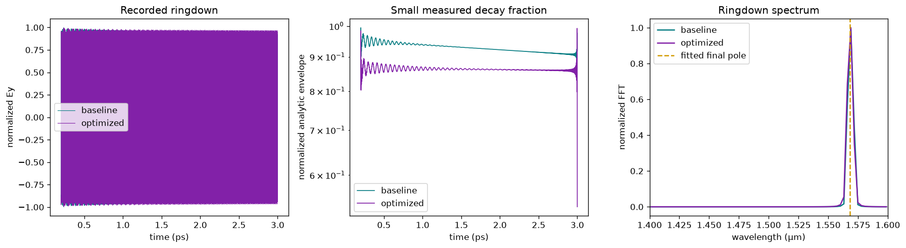
	unchanged baseline	optimized literal
wavelength (µm)	1.568706e+00	1.568299
independent Q	3.512530e+04	187133.234081
ResonanceFinder error	3.919232e-07	0.000005

9. Differentiable short fit versus independent long fit

The optimization fit sees only the first 6,000 post-source samples (three windows), whereas the held-out ResonanceFinder sees all 29,371 samples. Agreement does not have to be exact—the short fit is intentionally cheap—but both must track the same wavelength and the long independent result alone decides pass/fail.

short_fit = fdtdx.fit_resonance(
    jnp.asarray(final_sim.ringdown[:3 * SAMPLES_PER_WINDOW]),
    time_step=sample_dt,
    center_frequency=fdtdx.constants.c / 1.57e-6,
    samples_per_window=SAMPLES_PER_WINDOW,
    num_windows=3,
)
fit_table = pd.DataFrame({
    "differentiable 0.6 ps fit": [
        float(fdtdx.constants.c / short_fit.frequency * 1e6),
        float(short_fit.quality_factor), float(short_fit.residual),
        float(short_fit.window_consistency),
    ],
    "independent 2.8 ps fit": [
        final_pole["wavelength_um"], final_pole["Q"],
        final_pole["fit_error"], np.nan,
    ],
}, index=["wavelength (µm)", "Q", "fit residual/error", "window consistency"])
fit_table

	differentiable 0.6 ps fit	independent 2.8 ps fit
wavelength (µm)	1.568298	1.568299
Q	157462.078125	187133.234081
fit residual/error	0.000204	0.000005
window consistency	0.151263	NaN

10. Local FDTDX metrics

metrics = pd.Series({
    "unchanged baseline Q": baseline_pole["Q"],
    "required Q": 2 * baseline_pole["Q"],
    "mirror-completed control Q": MIRROR_COMPLETED_CONTROL_Q,
    "optimized literal Q": final_pole["Q"],
    "optimized / unchanged": final_pole["Q"] / baseline_pole["Q"],
    "optimized / completed control": final_pole["Q"] / MIRROR_COMPLETED_CONTROL_Q,
    "minimum silicon bridge (nm)": fabrication["minimum_silicon_gap_nm"],
    "minimum hole diameter (nm)": fabrication["minimum_hole_diameter_nm"],
    "fabrication violation (nm)": fabrication["fabrication_violation_nm"],
    "binary material fraction": 1.0,
}, name="measured value")
display(metrics.to_frame())
assert metrics["optimized / unchanged"] >= 2.0
assert metrics["optimized / completed control"] >= 1.0
assert metrics["fabrication violation (nm)"] == 0.0
print("PASS: literal inverse-designed Q exceeds both physical controls.")
print("uv run fdtdx-bench run --case invdes_nanobeam_cavity")

	measured value
unchanged baseline Q	35125.300715
required Q	70250.601430
mirror-completed control Q	92493.301338
optimized literal Q	187133.234081
optimized / unchanged	5.327591
optimized / completed control	2.023209
minimum silicon bridge (nm)	141.609818
minimum hole diameter (nm)	185.481277
fabrication violation (nm)	0.000000
binary material fraction	1.000000

PASS: literal inverse-designed Q exceeds both physical controls.
uv run fdtdx-bench run --case invdes_nanobeam_cavity

11. Independent Tidy3D verification of the same cylinders

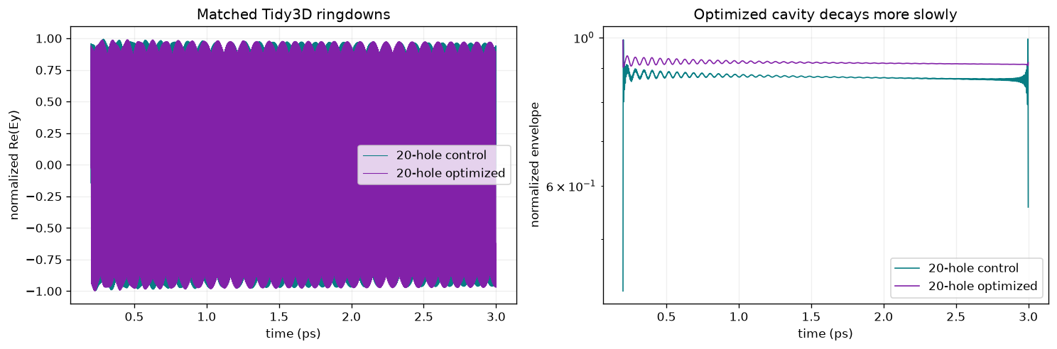
The fixed-count control and optimized arrays above were inserted into the trusted Tidy3D nanobeam builder without changing its 25 nm uniform grid, silicon/oxide materials, source, three time probes, 12-layer PML, (1, -1, 0) symmetry, or 3 ps runtime. Both Tidy3D scenes contain exactly 20 holes, so this ratio cannot benefit from adding mirror periods. The cloud solves are frozen here; executing this notebook reads their signals and does not submit a paid task.

tidy = np.load(tidy_validation_path, allow_pickle=True)
tidy_meta = json.loads(str(tidy["meta_json"]))

fig, axes = plt.subplots(1, 2, figsize=(12.5, 4.2))
for stem, label, color in (
    ("mirror_completed_control", "20-hole control", "#087d83"),
    ("optimized", "20-hole optimized", "#8221a8"),
):
    time_ps_tidy = tidy[f"{stem}_time_s"] * 1e12
    signal_tidy = np.asarray(tidy[f"{stem}_signal"])
    normalized = signal_tidy / np.max(np.abs(signal_tidy))
    envelope = np.abs(hilbert(np.real(signal_tidy)))
    axes[0].plot(time_ps_tidy[::8], np.real(normalized[::8]), lw=0.65,
                 label=label, color=color)
    axes[1].semilogy(time_ps_tidy[::12], (envelope / envelope.max())[::12],
                    lw=1.0, label=label, color=color)
axes[0].set(xlabel="time (ps)", ylabel="normalized Re(Ey)",
            title="Matched Tidy3D ringdowns")
axes[1].set(xlabel="time (ps)", ylabel="normalized envelope",
            title="Optimized cavity decays more slowly")
for ax in axes:
    ax.grid(alpha=0.2)
    ax.legend()
plt.tight_layout()
plt.show()

cross_solver = pd.DataFrame({
    "FDTDX": [
        MIRROR_COMPLETED_CONTROL_Q,
        final_pole["Q"],
        final_pole["Q"] / MIRROR_COMPLETED_CONTROL_Q,
    ],
    "Tidy3D": [
        float(tidy["mirror_completed_control_Q"][0]),
        float(tidy["optimized_Q"][0]),
        float(tidy["tidy3d_q_ratio"][0]),
    ],
}, index=["20-hole control Q", "20-hole optimized Q", "optimized / control"])
display(cross_solver)
print("Tidy3D control fit error:", float(tidy["mirror_completed_control_fit_error"][0]))
print("Tidy3D optimized fit error:", float(tidy["optimized_fit_error"][0]))
print("Tidy3D task IDs:", {name: values["task_id"] for name, values in tidy_meta["tasks"].items()})
print("Billed FlexCredits:", sum(values["actual_flexcredits"] for values in tidy_meta["tasks"].values()))
assert float(tidy["tidy3d_q_ratio"][0]) > 1.0

	FDTDX	Tidy3D
20-hole control Q	92493.301338	84246.788385
20-hole optimized Q	187133.234081	146677.821390
optimized / control	2.023209	1.741049

Tidy3D control fit error: 0.023585881021420136
Tidy3D optimized fit error: 0.001235640038273991
Tidy3D task IDs: {'mirror_completed_control': 'fdve-1b9cf912-868e-4779-a79d-8fe99e72b2a4', 'optimized': 'fdve-f63006bd-ae2e-490e-8506-ce3d0310e9b0'}
Billed FlexCredits: 0.09794087790122365

Interpretation

The unchanged eight-hole cavity reaches about \(3.5 imes10^4\). Automatic mirror completion removes an artificial leakage bottleneck and reaches about \(9.2 imes10^4\); that setup improvement is reported separately and is not attributed to the adjoint. One fitted-Q adjoint update then more than doubles the completed control in the independent literal solve, reaching about \(1.87 imes10^5\) or 5.3× the unchanged cavity. In the independent matched Tidy3D pair, the same shape change raises Q from 84,247 to 146,678, a 1.741× fixed-hole-count improvement. Tidy3D therefore confirms that the shape optimization works, while also showing that the present 25 nm FDTDX discretization overpredicts its magnitude (2.023× locally). The small center/radius shifts are physically resolved by both solvers’ subpixel interface treatments; this was a bounded 20-parameter shape optimization, not a pixel design.

For fabrication or publication, repeat across grid spacings, etch bias, sidewall angle, material dispersion, and multiple fitting windows. This notebook proves the requested GPU-native automatic-differentiation workflow and its held-out physical result; it does not claim that a single nominal design is robust to every process variation.