Dielectric metasurface absorber: R, T, and A

This notebook reconstructs one periodic THz unit cell from the official Tidy3D dielectric-metasurface example. It builds a lossy PDMS layer and dispersive Drude silicon cylinder, runs empty-cell normalization plus the device at three frequencies, plots the actual terminal field, and computes \(A=1-R-T\).

Imports and parameters

import os
os.environ.setdefault("XLA_PYTHON_CLIENT_PREALLOCATE", "false")
from time import perf_counter
import matplotlib.pyplot as plt
from matplotlib.patches import Rectangle
import numpy as np
import pandas as pd
import fdtdx
from IPython import get_ipython

from benchmarks.cases.device_metasurface_absorber.run import (
    DL, FREQUENCIES, HEIGHT, LZ, PERIOD, PML_LAYERS, RADIUS,
    SIM_TIME, SUBSTRATE_THICKNESS, THZ, UM, _build, _mean_flux,
)
from benchmarks.runners.fdtdx_util import run_scene

get_ipython().run_line_magic("matplotlib", "inline")
pd.Series({
    "period_um": PERIOD / UM,
    "cylinder_radius_um": RADIUS / UM,
    "cylinder_height_um": HEIGHT / UM,
    "PDMS_thickness_um": SUBSTRATE_THICKNESS / UM,
    "frequencies_THz": tuple(FREQUENCIES / THZ),
    "grid_pitch_um": DL / UM,
    "maximum_time_ps": SIM_TIME * 1e12,
    "PML_cells": PML_LAYERS,
}, name="value").to_frame()

	value
period_um	330.0
cylinder_radius_um	106.0
cylinder_height_um	85.0
PDMS_thickness_um	8.0
frequencies_THz	(0.5, 0.6, 0.7)
grid_pitch_um	5.0
maximum_time_ps	40.0
PML_cells	12

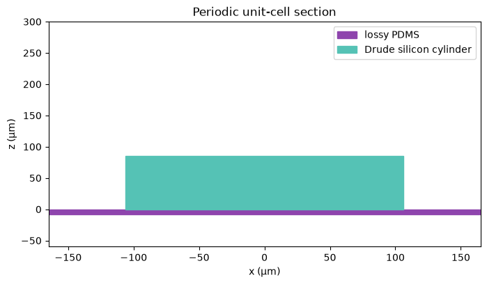
1. Geometry and material stack

fig, ax = plt.subplots(figsize=(8, 4.2))
ax.add_patch(Rectangle((-PERIOD / UM / 2, -SUBSTRATE_THICKNESS / UM), PERIOD / UM, SUBSTRATE_THICKNESS / UM, color="#8e44ad", label="lossy PDMS"))
ax.add_patch(Rectangle((-RADIUS / UM, 0), 2 * RADIUS / UM, HEIGHT / UM, color="#55c2b5", label="Drude silicon cylinder"))
ax.set(xlabel="x (µm)", ylabel="z (µm)", title="Periodic unit-cell section", xlim=(-PERIOD / UM / 2, PERIOD / UM / 2), ylim=(-60, 300))
ax.legend(); plt.show()

2. Build and plot the 0.6 THz scene

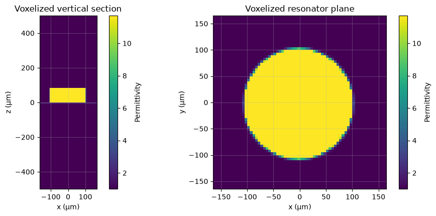
preview_objects, preview_arrays, preview_config = run_scene(*_build(0.6 * THZ, with_device=True), seed=0)
print(f"Yee grid: {preview_objects.volume.grid_shape}")
print(f"Time steps per frequency: {preview_config.time_steps_total:,}")
fig, axes = plt.subplots(1, 2, figsize=(11, 4.4))
fdtdx.plot_material_from_side(preview_config, preview_arrays, "y", position=0.0, ax=axes[0], plot_legend=True)
fdtdx.plot_material_from_side(preview_config, preview_arrays, "z", position=20 * UM, ax=axes[1], plot_legend=True)
axes[0].set_title("Voxelized vertical section")
axes[1].set_title("Voxelized resonator plane")
plt.tight_layout(); plt.show()

Yee grid: (66, 66, 200)
Time steps per frequency: 4,196

3. Run empty and device cells

reflection, transmission = [], []
executed = {}
started = perf_counter()
for frequency in FREQUENCIES:
    _, empty, empty_config = run_scene(*_build(float(frequency), with_device=False), seed=0)
    objects, device, device_config = run_scene(*_build(float(frequency), with_device=True), seed=0)
    reference_power = _mean_flux(empty, "flux_t", float(frequency))
    reflection.append(_mean_flux(device, "flux_r", float(frequency)) / reference_power)
    transmission.append(_mean_flux(device, "flux_t", float(frequency)) / reference_power)
    executed[float(frequency)] = (objects, device, device_config)
print(f"Six local FDTDX runs: {perf_counter() - started:.1f} s")

R = np.asarray(reflection)
T = np.asarray(transmission)
A = 1 - R - T

Six local FDTDX runs: 26.9 s

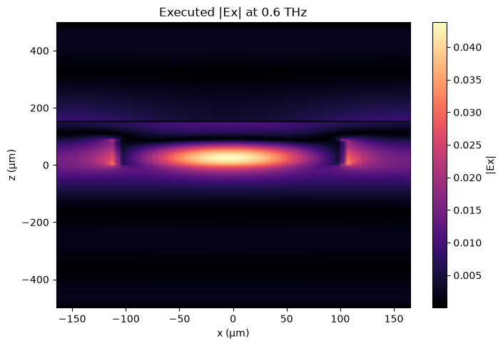
4. Plot an actual simulated field

objects, device, device_config = executed[float(FREQUENCIES[1])]
ex = np.asarray(device.fields.E[0])
ex_xz = ex[:, ex.shape[1] // 2, :]
fig, ax = plt.subplots(figsize=(8, 5.2))
image = ax.imshow(np.abs(ex_xz).T, origin="lower", cmap="magma", aspect="auto", extent=(-PERIOD / UM / 2, PERIOD / UM / 2, -LZ / UM / 2, LZ / UM / 2))
ax.set(xlabel="x (µm)", ylabel="z (µm)", title="Executed |Ex| at 0.6 THz")
fig.colorbar(image, ax=ax, label="|Ex|"); plt.show()

5. Reflection, transmission, and absorption

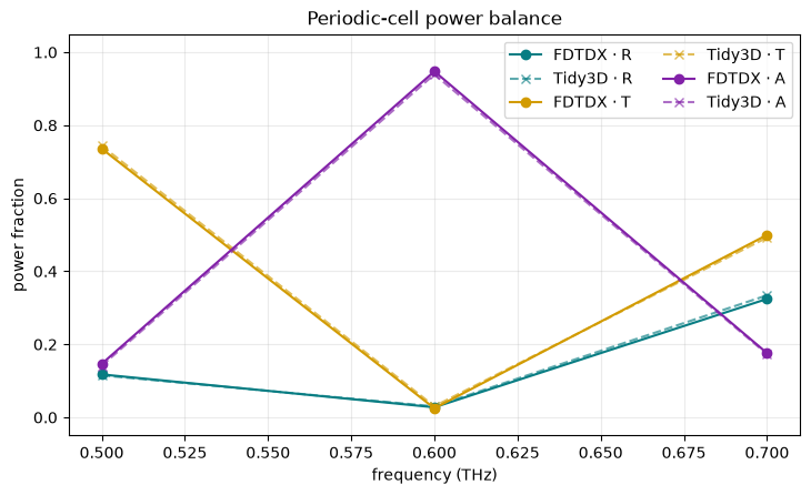
frequencies_thz = FREQUENCIES / THZ
golden = np.load("benchmarks/goldens/device_metasurface_absorber.npz", allow_pickle=True)
fig, ax = plt.subplots(figsize=(8.5, 4.7))
for name, values, color in (("R", R, "#087d83"), ("T", T, "#d29b00"), ("A", A, "#8221a8")):
    ax.plot(frequencies_thz, values, "o-", color=color, label=f"FDTDX · {name}")
    ax.plot(frequencies_thz, golden[name], "x--", color=color, alpha=0.65, label=f"Tidy3D · {name}")
ax.set(xlabel="frequency (THz)", ylabel="power fraction", title="Periodic-cell power balance", ylim=(-0.05, 1.05))
ax.grid(alpha=0.25); ax.legend(ncol=2); plt.show()
pd.DataFrame({"frequency_THz": frequencies_thz, "R": R, "T": T, "A": A, "R+T+A": R + T + A})

	frequency_THz	R	T	A	R+T+A
0	0.5	0.117592	0.735854	0.146554	1.0
1	0.6	0.027566	0.024862	0.947572	1.0
2	0.7	0.324380	0.499590	0.176031	1.0

Reproduce

The empty-cell run is essential: it makes source amplitude and finite grid area cancel from R and T.

print("uv run fdtdx-bench run --case device_metasurface_absorber")

uv run fdtdx-bench run --case device_metasurface_absorber