Maxwell on a Yee grid

FDTD replaces spatial curls with finite differences and advances electric and magnetic fields in a leapfrog sequence. For linear media, the continuous equations are

\[ \nabla\times\mathbf E=-\frac{\partial\mathbf B}{\partial t},\qquad \nabla\times\mathbf H=\frac{\partial\mathbf D}{\partial t}+\mathbf J, \]

with constitutive relations \(\mathbf D=\boldsymbol\varepsilon\mathbf E\) and \(\mathbf B=\boldsymbol\mu\mathbf H\). FDTDX stores the three vector components on offset locations in each cell so a discrete curl naturally connects neighboring samples.

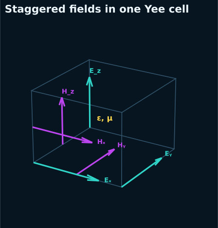
Electric components live on edges; magnetic components occupy complementary staggered locations. Material values are mapped onto the corresponding component locations.

Leapfrog update

Ignoring conductivity and PML terms for the moment, one time step is conceptually

\[ \mathbf H^{n+1/2}=\mathbf H^{n-1/2}-\Delta t\,\boldsymbol\mu^{-1}\nabla_h\times\mathbf E^n, \]

\[ \mathbf E^{n+1}=\mathbf E^n+\Delta t\,\boldsymbol\varepsilon^{-1}\left(\nabla_h\times\mathbf H^{n+1/2}-\mathbf J^{n+1/2}\right). \]

FDTDX represents inverse material tensors because those are applied directly in the update. Conductivity, dispersive-pole state, and PML auxiliary fields add local terms but preserve the same rhythm.

Stability is necessary, not sufficient

For a uniform 3D grid, a familiar Courant bound is

\[ \Delta t \leq \frac{S}{c\sqrt{\Delta x^{-2}+\Delta y^{-2}+\Delta z^{-2}}}, \qquad S\leq1. \]

Staying below it prevents the ordinary Yee scheme from diverging. It does not guarantee accuracy: numerical phase velocity depends on direction and cells per wavelength. Interfaces introduce staircasing error, and resonances demand enough runtime to resolve narrow spectral structure.

Why FDTD suits JAX

Each time step is a regular stencil over dense arrays. JAX compiles that array program for GPU, CPU, or TPU; lax.scan/loop constructs avoid Python overhead; and the same program participates in automatic differentiation. Static shapes are important: changing a grid dimension causes recompilation.

Precision and scaling

Most benchmarks use float32, which is efficient on consumer GPUs and accurate enough when discretization error dominates. Use nondimensional diagnostics—relative energy decay, normalized mode power, \(R+T\), convergence with resolution—rather than judging raw array magnitudes alone.