Your first simulation

Every FDTDX run follows the same arc: configure the numerical grid, declare objects, constrain their placement, materialize arrays, then advance Maxwell’s equations.

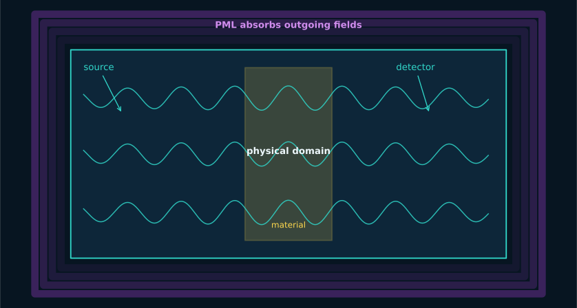
A minimal scene still has four distinct roles: domain, boundary, excitation, and observation.

1. Choose physical scales

Suppose a plane wave at wavelength \(\lambda_0\) illuminates a dielectric slab. Choose the spatial step from the shortest wavelength in material, not just the vacuum wavelength:

\[ \Delta \lesssim \frac{\lambda_0}{N_\lambda n_{\max}}, \qquad N_\lambda \approx 10\text{–}20. \]

The Courant condition then limits the time step. SimulationConfig computes this consistently from the grid and courant_factor.

import fdtdx
import jax.numpy as jnp

config = fdtdx.SimulationConfig(
    time=120e-15,
    grid=fdtdx.UniformGrid(spacing=40e-9),
    dtype=jnp.float32,
    courant_factor=0.99,
)
volume = fdtdx.SimulationVolume(partial_grid_shape=(160, 8, 8))

2. Declare rather than mutate

Materials, sources, and detectors are objects. Placement constraints express how they sit relative to the simulation volume or to one another. place_objects solves those constraints, allocates arrays, and returns an immutable ObjectContainer.

slab = fdtdx.UniformMaterialObject(
    name="slab",
    partial_grid_shape=(24, 8, 8),
    material=fdtdx.Material(permittivity=4.0),
)

source = fdtdx.UniformPlaneSource(
    name="source",
    partial_grid_shape=(1, 8, 8),
    wave_character=fdtdx.WaveCharacter(wavelength=1.55e-6),
    direction="+",
    fixed_E_polarization_vector=(0, 1, 0),
)

The exact source signature and placement constraints used by the current, tested slab experiment live in benchmarks/cases/analytical_dielectric_slab/run.py. It is deliberately treated as executable documentation:

uv run fdtdx-bench run --case analytical_dielectric_slab

3. Apply parameters, then run

place_objects(...) returns (objects, arrays, params, config, info). apply_params(...) maps parameter values into material arrays. A forward solve then evolves E, H, boundary auxiliary fields, and detector state:

import jax

key = jax.random.PRNGKey(0)
objects, arrays, params, config, info = fdtdx.place_objects(
    object_list=scene,
    config=config,
    constraints=constraints,
    key=key,
)
arrays, objects, info = fdtdx.apply_params(arrays, objects, params, key)

final_state = fdtdx.run_fdtd(
    arrays=arrays,
    objects=objects,
    config=config,
    key=key,
)

API detail

FDTDX evolves quickly. Prefer the tested runners and the API map when copying a complete program; the fragments above emphasize structure and omit case-specific boundary and detector setup.

4. Check physics before scaling up

A plausible-looking field is not enough. For this slab, check reflected and transmitted flux against Fresnel theory and verify \(R+T\approx1\) for a lossless material. The suite records both quantities and their tolerances.

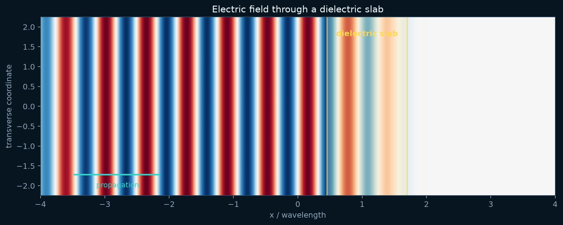
The wavelength changes inside the dielectric while tangential field continuity governs reflection and transmission.

Next: build the right mental model, then follow the fields and boundaries tutorial.