Shape optimization of a remote-atom silicon cavity

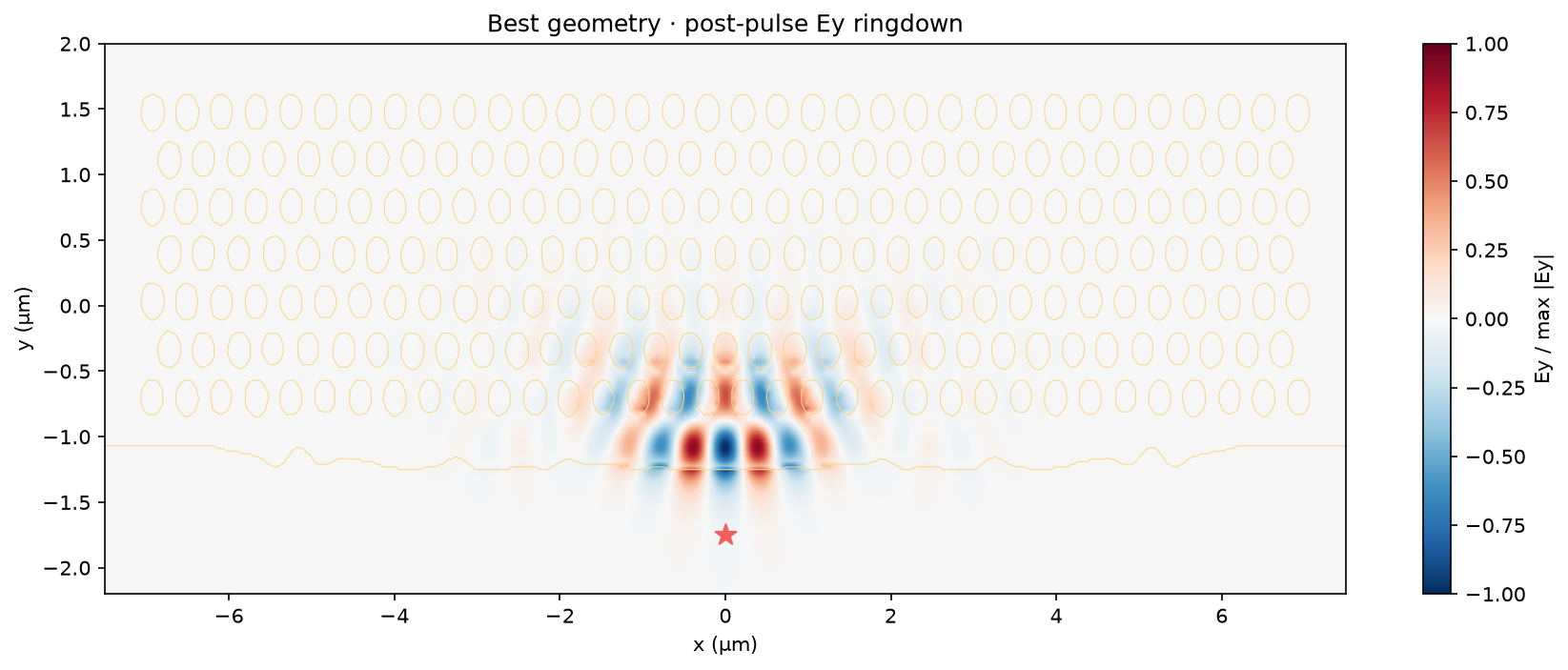
This executed example freezes the best accepted geometry from the GPU-native shifted-LDOS optimization of the unloaded Zhang et al. semi-2D cavity. An Ey-oriented atom is exactly 500 nm from the closest silicon point. The design is always a binary 220 nm single-etch extrusion: the optimizer moves a smooth membrane edge and the positions and radii of all retained holes.

The headline values below are a deterministic replay on the 40 nm optimization grid, not the pending 20 nm independent validation. Rejected trust-region trials remain visible in the history and are not presented as device states.

1. Parameters and frozen evidence

%matplotlib inline

from pathlib import Path
from io import BytesIO
import json
import numpy as np
import pandas as pd
import matplotlib.pyplot as plt
from matplotlib.patches import Circle
from IPython.display import Image, display

def show_figure(fig):
    buffer = BytesIO()
    fig.savefig(buffer, format="png", dpi=150, bbox_inches="tight")
    plt.close(fig)
    display(Image(data=buffer.getvalue()))

from benchmarks.cases.invdes_paper_semi2d_atom_ldos import geometry, run

ROOT = Path.cwd()
artifact_path = ROOT / "benchmarks/artifacts/paper_semi2d_atom_ldos_silicon_best_v1.npz"
with np.load(artifact_path, allow_pickle=False) as stored:
    frozen = {key: stored[key] for key in stored.files}

metrics = json.loads(str(frozen["metrics_json"]))
fabrication = json.loads(str(frozen["fabrication_json"]))
history = json.loads(str(frozen["history_json"]))
parameters = run.DEVICE_PARAMETERS

pd.Series({
    "material": "silicon (n=3.46)",
    "target wavelength": "1.547 µm",
    "slab thickness": f"{parameters.slab_thickness_um:.3f} µm",
    "atom clearance": f"{fabrication['minimum_atom_material_distance_um']:.3f} µm",
    "physical / independent holes": f"{fabrication['physical_hole_count']} / {fabrication['independent_hole_count']}",
    "shape controls": fabrication["control_count"],
    "symmetry": tuple(int(v) for v in frozen["symmetry"]),
    "grid spacing": f"{float(frozen['grid_spacing_nm']):.0f} nm",
    "controls SHA-256": str(frozen["controls_sha256"]),
}, name="value")

material                                                         silicon (n=3.46)
target wavelength                                                        1.547 µm
slab thickness                                                           0.220 µm
atom clearance                                                           0.500 µm
physical / independent holes                                            235 / 119
shape controls                                                                379
symmetry                                                                (1, 0, 1)
grid spacing                                                                40 nm
controls SHA-256                e6da737c3f981b3fdfc27c21b4aa5eaa487b1b9f7e1e25...
Name: value, dtype: object

2. Geometry setting and literal geometry

best_controls = np.asarray(frozen["best_controls"], dtype=np.float32)
zero_controls = np.asarray(frozen["zero_controls"], dtype=np.float32)
initial = geometry.decode_controls(zero_controls, parameters)
optimized = geometry.decode_controls(best_controls, parameters)
initial_holes, initial_radii = geometry.full_holes_um(initial)
optimized_holes, optimized_radii = geometry.full_holes_um(optimized)

x = np.linspace(-7.2, 7.2, 2400)
initial_edge = np.asarray(geometry.edge_y_um(x, initial, parameters))
optimized_edge = np.asarray(geometry.edge_y_um(x, optimized, parameters))
atom_x, atom_y, _ = parameters.atom_position_um

fig, axes = plt.subplots(1, 2, figsize=(15, 5), constrained_layout=True)
for ax, decoded_edge, holes, radii, title in (
    (axes[0], initial_edge, initial_holes, initial_radii, "Cold start"),
    (axes[1], optimized_edge, optimized_holes, optimized_radii, "Best accepted geometry"),
):
    ax.fill_between(x, decoded_edge, 2.0, color="#d8aa48", alpha=0.88, label="silicon")
    for center, radius in zip(holes, radii, strict=True):
        ax.add_patch(Circle(center, radius, facecolor="#101820", edgecolor="#ffe0a0", lw=0.25))
    ax.scatter([atom_x], [atom_y], marker="*", s=130, color="#f25f5c", zorder=5, label="Ey atom")
    ax.plot([0, 0], [atom_y, atom_y + 0.5], color="#42c6d7", lw=2)
    ax.set(xlim=(-7.2, 7.2), ylim=(-2.1, 1.8), xlabel="x (µm)", ylabel="y (µm)", title=title)
    ax.set_aspect("equal")
axes[0].legend(loc="lower right")
show_figure(fig)

The hard center clearance is unchanged. Away from the center, 24 effective edge controls apodize the bulge. Every one of the 119 x-mirror hole representatives has an independent radius and y position; the 116 holes off the mirror plane also move in x.

layout = run.LAYOUT
base = geometry.decode_controls(zero_controls, parameters)
best = geometry.decode_controls(best_controls, parameters)
changes_nm = pd.Series({
    "maximum |edge displacement|": 1e3 * np.max(np.abs(np.asarray(best.bulge_clearances_um) - np.asarray(base.bulge_clearances_um))),
    "maximum |hole x displacement|": 1e3 * np.max(np.abs(np.asarray(best.hole_x_um) - np.asarray(base.hole_x_um))),
    "maximum |hole y displacement|": 1e3 * np.max(np.abs(np.asarray(best.hole_y_um) - np.asarray(base.hole_y_um))),
    "maximum |radius change|": 1e3 * np.max(np.abs(np.asarray(best.hole_radii_um) - np.asarray(base.hole_radii_um))),
}, name="nanometres")
changes_nm.to_frame()

	nanometres
maximum |edge displacement|	87.281403
maximum |hole x displacement|	8.715153
maximum |hole y displacement|	9.226322
maximum |radius change|	9.201750

3. Simulation and differentiable shifted-pole objective

simulation = {
    "full grid": tuple(int(v) for v in frozen["domain_cells_full"]),
    "simulated grid after x/z symmetry": (205, 124, 32),
    "time window": f"{float(frozen['run_time_ps']):.1f} ps",
    "source": "Ey point dipole at the atom",
    "boundary": "12-cell PML",
    "objective": "log[1 + (3/4π²) λ*³ Q*/Vatom]",
    "Q estimator": "minimum of local-field and total-energy decay Q",
    "pole guard": "3% atomic-frequency branch window plus fit-health gates",
}
pd.Series(simulation, name="setting")

full grid                                                               (410, 124, 64)
simulated grid after x/z symmetry                                       (205, 124, 32)
time window                                                                     5.0 ps
source                                                     Ey point dipole at the atom
boundary                                                                   12-cell PML
objective                                                log[1 + (3/4π²) λ*³ Q*/Vatom]
Q estimator                            minimum of local-field and total-energy decay Q
pole guard                           3% atomic-frequency branch window plus fit-hea...
Name: setting, dtype: object

# This is the exact expensive replay used to create the frozen artifact.
# It is shown for reproducibility but not rerun while rendering the docs.
def replay_best_on_gpu(best_controls, tracking_frequency_hz):
    import jax
    import jax.numpy as jnp
    setup_data = run.setup()
    evaluate = jax.jit(
        lambda candidate: run._objective(
            candidate,
            jnp.asarray(tracking_frequency_hz, dtype=jnp.float32),
            jnp.asarray(1, dtype=jnp.int32),
            setup_data,
        )
    )
    return evaluate(jnp.asarray(best_controls))

print("Frozen artifact contains the output of this forward replay on the best accepted controls.")

Frozen artifact contains the output of this forward replay on the best accepted controls.

4. Optimization history

iteration = np.asarray([row["iteration"] for row in history])
ldos = np.asarray([row["shifted_ldos"] for row in history])
quality = np.asarray([row["quality_factor"] for row in history])
accepted = np.asarray([bool(row["accepted"]) for row in history])

fig, axes = plt.subplots(1, 2, figsize=(13, 4.3), constrained_layout=True)
for ax, values, ylabel in ((axes[0], ldos, "shifted LDOS / vacuum"), (axes[1], quality, "conservative Q")):
    ax.plot(iteration, values, "--", color="#7c8b96", alpha=0.45, lw=1)
    ax.plot(iteration[accepted], values[accepted], "o", color="#50c878", ms=4, label="accepted")
    ax.plot(iteration[~accepted], values[~accepted], "x", color="#f25f5c", ms=5, label="rejected trial")
    ax.set(xlabel="FDTD evaluation", ylabel=ylabel)
    ax.grid(alpha=0.2)
axes[1].set_yscale("log")
axes[0].legend()
show_figure(fig)

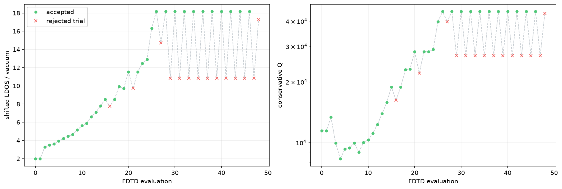
The late alternating points are deliberately retained. They exposed a rollback defect that regenerated one rejected Adam proposal from the same trusted leader. The campaign was stopped, its best geometry frozen, and the optimizer was hardened with geometric half-step backtracking. No rejected point changed the saved device.

5. Paired electric field

field_positive = np.asarray(frozen["ey_xy"], dtype=float)
fill_positive = np.asarray(frozen["silicon_fill_xy"], dtype=float)
x_positive = np.asarray(frozen["x_um"], dtype=float)
y = np.asarray(frozen["y_um"], dtype=float)
x_full = np.concatenate((-x_positive[::-1], x_positive))
field = np.concatenate((field_positive[::-1], field_positive), axis=0)
fill = np.concatenate((fill_positive[::-1], fill_positive), axis=0)
field /= max(np.max(np.abs(field)), 1e-30)

fig, ax = plt.subplots(figsize=(14, 5))
image = ax.imshow(field.T, origin="lower", extent=(x_full[0], x_full[-1], y[0], y[-1]),
                  cmap="RdBu_r", vmin=-1, vmax=1, interpolation="bilinear", aspect="auto")
ax.contour(x_full, y, fill.T, levels=(0.5,), colors=("#f8d78c",), linewidths=0.5)
ax.scatter([atom_x], [atom_y], marker="*", s=120, color="#f25f5c", zorder=5)
ax.set(xlim=(-7.5, 7.5), ylim=(-2.2, 2.0), xlabel="x (µm)", ylabel="y (µm)",
       title="Best geometry · post-pulse Ey ringdown")
fig.colorbar(image, ax=ax, label="Ey / max |Ey|")
show_figure(fig)

6. Analysis

pd.DataFrame({
    "quantity": [
        "shifted peak LDOS / vacuum", "resonant Purcell contribution", "conservative Q",
        "field-decay Q", "energy-decay Q", "atom-oriented mode volume", "pole wavelength",
        "field fit residual", "energy fit residual", "atom detuning",
    ],
    "value": [
        metrics["shifted_ldos"], metrics["purcell_factor"], metrics["quality_factor"],
        metrics["field_quality_factor"], metrics["energy_quality_factor"],
        f"{metrics['mode_volume_um3']:.3f} µm³", f"{metrics['wavelength_um']:.6f} µm",
        metrics["fit_residual"], metrics["energy_fit_residual"],
        f"{100 * metrics['detuning_fraction']:.4f}%",
    ],
}).set_index("quantity")

	value
quantity
shifted peak LDOS / vacuum	18.165806
resonant Purcell contribution	17.165806
conservative Q	44666.714844
field-decay Q	52881.746094
energy-decay Q	44666.714844
atom-oriented mode volume	715.888 µm³
pole wavelength	1.535517 µm
field fit residual	0.000012
energy fit residual	0.003441
atom detuning	0.7478%

The replay gives LDOS 18.166 and conservative Q 44,667. The field and energy estimators agree to within 18.4%; the reported Q is their lower value. The optimized atom-oriented mode volume is 715.89 µm³. The fitted-pole value is

\[1 + \frac{3}{4\pi^2}\frac{\lambda_*^3Q_*}{V_\mathrm{atom}}.\]

This is strong optimization evidence, but it is not silently promoted to a fine-grid result. A new 20 nm long-ringdown replay and matched-vacuum LDOS are still required for an independently validated performance claim.