Polarization splitter-rotator: TE/TM routing

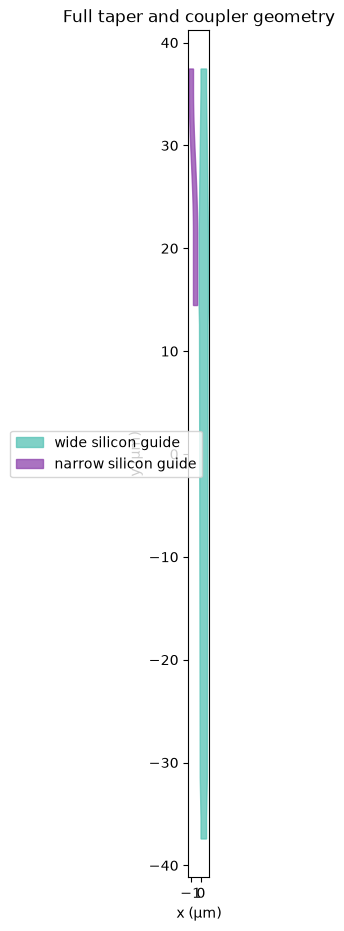
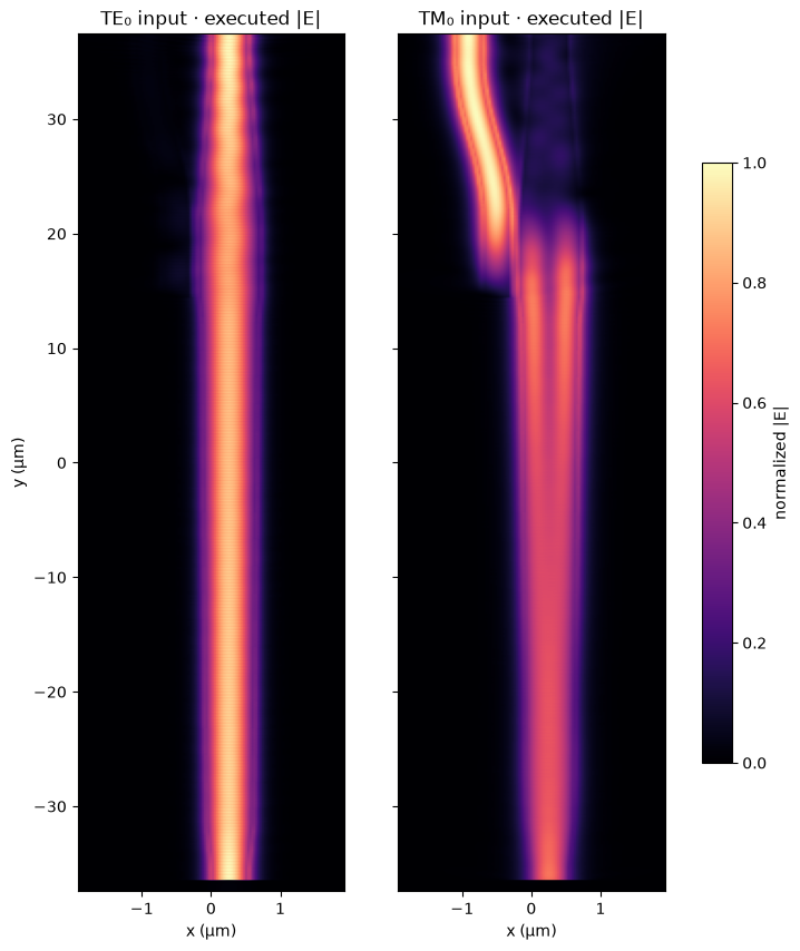
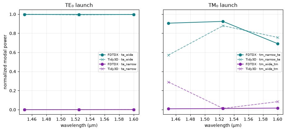
This notebook reconstructs the full 44 µm asymmetric taper and directional-coupler section from the official Tidy3D PSR example. Separate TE₀ and TM₀ launches are run through the same geometry; actual field phasors and desired/leakage port spectra are plotted for both inputs.

Imports and parameters

import os
os.environ.setdefault("XLA_PYTHON_CLIENT_PREALLOCATE", "false")
from time import perf_counter
import matplotlib.pyplot as plt
import numpy as np
import pandas as pd
import fdtdx
from IPython import get_ipython

from benchmarks.cases.device_polarization_splitter_rotator.run import (
    DL_UM, DOMAIN_UM, PML_LAYERS, RUN_TIME, UM, WAVELENGTH0_UM,
    WAVELENGTHS_UM, _scene,
)
from benchmarks.device_geometry import polarization_splitter_rotator_vertices_um

get_ipython().run_line_magic("matplotlib", "inline")
pd.Series({
    "domain_um": DOMAIN_UM,
    "wavelengths_um": WAVELENGTHS_UM,
    "center_wavelength_um": WAVELENGTH0_UM,
    "axis_grid_pitch_um": DL_UM,
    "maximum_time_ps": RUN_TIME * 1e12,
    "PML_cells": PML_LAYERS,
}, name="value").to_frame()

	value
domain_um	(3.855, 74.86666666666666, 1.4)
wavelengths_um	(1.45, 1.525, 1.6)
center_wavelength_um	1.525
axis_grid_pitch_um	(0.03, 0.04, 0.03)
maximum_time_ps	2.0
PML_cells	8

1. Exact asymmetric geometry

wide, narrow = polarization_splitter_rotator_vertices_um()
fig, ax = plt.subplots(figsize=(5.5, 11))
ax.fill(wide[:, 0], wide[:, 1], color="#55c2b5", alpha=0.75, label="wide silicon guide")
ax.fill(narrow[:, 0], narrow[:, 1], color="#8e44ad", alpha=0.75, label="narrow silicon guide")
ax.set(xlabel="x (µm)", ylabel="y (µm)", title="Full taper and coupler geometry", aspect="equal")
ax.legend(); plt.show()

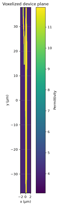
2. Build TE and TM scenes and inspect voxelization

scenes = {polarization: _scene(polarization, 1.0, record_field=True) for polarization in ("te", "tm")}
objects_te, arrays_te, config_te, _ = scenes["te"]
print(f"Anisotropic Yee grid: {objects_te.volume.grid_shape}")
print(f"Time-step ceiling per launch: {config_te.time_steps_total:,}")
fig, ax = plt.subplots(figsize=(5.5, 10))
fdtdx.plot_material_from_side(config_te, arrays_te, "z", position=0.0, ax=ax, plot_legend=True)
ax.set_title("Voxelized device plane"); plt.show()

Anisotropic Yee grid: (145, 1888, 63)
Time-step ceiling per launch: 32,318

3. Run the two input polarizations

results, states = {}, {}
started = perf_counter()
for polarization, (objects, arrays, config, output_ports) in scenes.items():
    results[polarization], states[polarization] = fdtdx.calculate_sparam(
        objects, arrays, config, "input", show_progress=False
    )
print(f"Two local FDTDX runs: {perf_counter() - started:.1f} s")

Two local FDTDX runs: 491.4 s

4. Plot the actual TE and TM field responses

fig, axes = plt.subplots(1, 2, figsize=(8.5, 10), sharex=True, sharey=True)
for ax, polarization in zip(axes, ("te", "tm"), strict=True):
    phasor = np.asarray(states[polarization]["field_xy"]["phasor"])[0, 0, :3]
    magnitude = np.sqrt(np.sum(np.abs(phasor) ** 2, axis=0)).squeeze()
    magnitude /= magnitude.max() + 1e-30
    image = ax.imshow(magnitude.T, origin="lower", cmap="magma", aspect="auto", extent=(-DOMAIN_UM[0] / 2, DOMAIN_UM[0] / 2, -DOMAIN_UM[1] / 2, DOMAIN_UM[1] / 2), vmin=0, vmax=1)
    ax.set(title=f"{polarization.upper()}₀ input · executed |E|", xlabel="x (µm)")
axes[0].set_ylabel("y (µm)")
fig.colorbar(image, ax=axes, label="normalized |E|", shrink=0.7)
plt.show()

5. Desired conversion and leakage spectra

port_names = {
    "te": ("te_wide", "te_narrow"),
    "tm": ("tm_narrow_te", "tm_wide_tm"),
}
powers = {}
for polarization, names in port_names.items():
    for name in names:
        powers[name] = np.abs(np.asarray(results[polarization][(name, "input")]).squeeze()) ** 2

golden = np.load("benchmarks/goldens/device_polarization_splitter_rotator.npz", allow_pickle=True)
wavelengths = np.asarray(WAVELENGTHS_UM)
fig, axes = plt.subplots(1, 2, figsize=(11, 4.4), sharey=True)
for ax, polarization in zip(axes, ("te", "tm"), strict=True):
    for name, color in zip(port_names[polarization], ("#087d83", "#8221a8"), strict=True):
        ax.plot(wavelengths, powers[name], "o-", color=color, label=f"FDTDX · {name}")
        ax.plot(wavelengths, golden[name], "x--", color=color, alpha=0.65, label=f"Tidy3D · {name}")
    ax.set(title=f"{polarization.upper()}₀ launch", xlabel="wavelength (µm)")
    ax.grid(alpha=0.25); ax.legend(fontsize=7)
axes[0].set_ylabel("normalized modal power")
plt.show()
pd.DataFrame({"wavelength_um": wavelengths, **powers})

	wavelength_um	te_wide	te_narrow	tm_narrow_te	tm_wide_tm
0	1.450	0.996876	0.000260	0.906050	0.009447
1	1.525	0.997406	0.000576	0.924553	0.012085
2	1.600	0.996504	0.001184	0.692314	0.016446

Reproduce

The anisotropic mesh resolves the 150 nm lateral gap and 220 nm layer while keeping the 75 µm propagation axis affordable.

print("uv run fdtdx-bench run --case device_polarization_splitter_rotator")

uv run fdtdx-bench run --case device_polarization_splitter_rotator