Inverse-designed four-channel wavelength demultiplexer

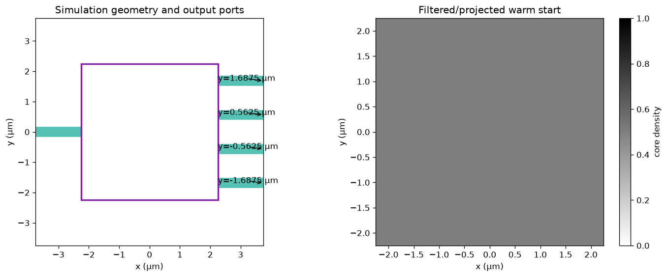
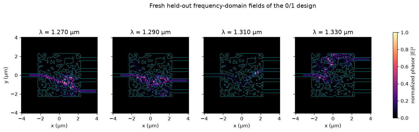
This executable notebook follows the corresponding official Tidy3D autograd tutorial: define the wavelength-dependent objective, plot the device and starting parameters, run topology optimization through differentiable FDTD, inspect the projected best design and a fresh best-design field solve, then analyze its spectrum. The objective is to route 1.27, 1.29, 1.31, and 1.33 µm into four separate outputs.

Imports and accelerator

import os
os.environ.setdefault("XLA_PYTHON_CLIENT_PREALLOCATE", "false")
import json
from pathlib import Path
from time import perf_counter
import warnings
import matplotlib.pyplot as plt
from matplotlib.patches import Rectangle
import numpy as np
import pandas as pd
import jax
import yaml
from IPython import get_ipython

from benchmarks.invdes_spectral_runner import (
    SPECS, _filter_project, initial_density, optimize_spectral_device,
    simulate_spectral_design,
)

get_ipython().run_line_magic("matplotlib", "inline")
warnings.filterwarnings("ignore", category=FutureWarning, module=r"tidy3d\.components\.mode")
plt.rcParams.update({"figure.figsize": (9, 4.5), "figure.dpi": 120})
CASE_ID = "invdes_wdm"
spec = SPECS[CASE_ID]
meta = yaml.safe_load(Path(f"benchmarks/cases/{CASE_ID}/case.yaml").read_text())
print(f"JAX devices: {jax.devices()}")

JAX devices: [CudaDevice(id=0)]

1. Physical, spectral, and optimization parameters

pd.Series({
    "objective": meta["invdes"]["objective"],
    "wavelengths_um": spec.wavelengths_um,
    "design_region_um": spec.design_um,
    "design_parameters": spec.parameter_shape,
    "FDTD_grid_pitch_um": spec.dl_um,
    "output_y_um": spec.output_y_um,
    "core_permittivity": spec.eps_core,
    "Adam_learning_rate": spec.learning_rate,
    "projection_beta": (1.0, spec.beta_max),
    "minimum_feature_radius_um": spec.feature_radius_um,
    "automatic_update_cap": meta["invdes"]["max_iterations"],
    "Tidy3D_updates": meta["invdes"]["ref_iterations"],
}, name="value").to_frame()

	value
objective	smooth-min channel routing minus off-channel l...
wavelengths_um	(1.2747924528301886, 1.272391713747646, 1.27, ...
design_region_um	(4.5, 4.5)
design_parameters	(300, 300)
FDTD_grid_pitch_um	0.05
output_y_um	(-1.6875, -0.5625, 0.5625, 1.6875)
core_permittivity	12.1801
Adam_learning_rate	0.05
projection_beta	(1.0, 50.0)
minimum_feature_radius_um	0.1
automatic_update_cap	150
Tidy3D_updates	50

2. Geometry, ports, and initial density

density0 = initial_density(spec)
projected0 = np.asarray(_filter_project(jax.numpy.asarray(density0), 1.0, spec))
dx, dy = spec.design_um
cx, cy = spec.core_um
width = spec.waveguide_width_um

fig, axes = plt.subplots(1, 2, figsize=(12, 4.8))
ax = axes[0]
left_length = (cx - dx) / 2
ax.add_patch(Rectangle((-cx / 2, -width / 2), left_length, width, color="#55c2b5"))
for output_y in spec.output_y_um:
    ax.add_patch(Rectangle((dx / 2, output_y - width / 2), left_length, width, color="#55c2b5"))
    ax.annotate(f"y={output_y:g} µm", (cx / 2, output_y), (dx / 2, output_y), arrowprops={"arrowstyle": "->"})
ax.add_patch(Rectangle((-dx / 2, -dy / 2), dx, dy, facecolor="none", edgecolor="#8221a8", lw=2))
ax.set(xlim=(-cx / 2, cx / 2), ylim=(-cy / 2, cy / 2), aspect="equal",
       xlabel="x (µm)", ylabel="y (µm)", title="Simulation geometry and output ports")

image = axes[1].imshow(projected0.T, origin="lower", extent=(-dx / 2, dx / 2, -dy / 2, dy / 2),
                       cmap="gray_r", vmin=0, vmax=1, aspect="equal")
axes[1].set(xlabel="x (µm)", ylabel="y (µm)", title="Filtered/projected warm start")
fig.colorbar(image, ax=axes[1], label="core density")
plt.tight_layout(); plt.show()

3. Run differentiable spectral optimization

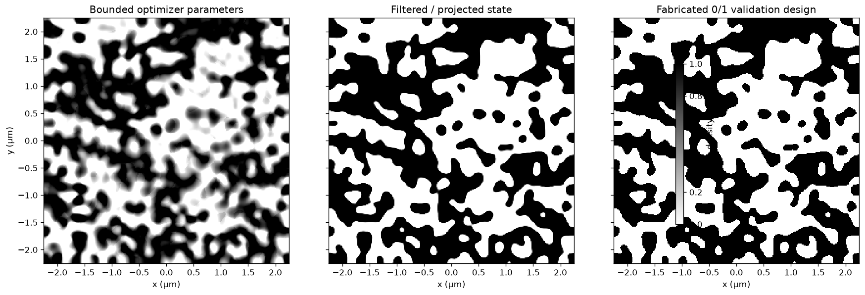
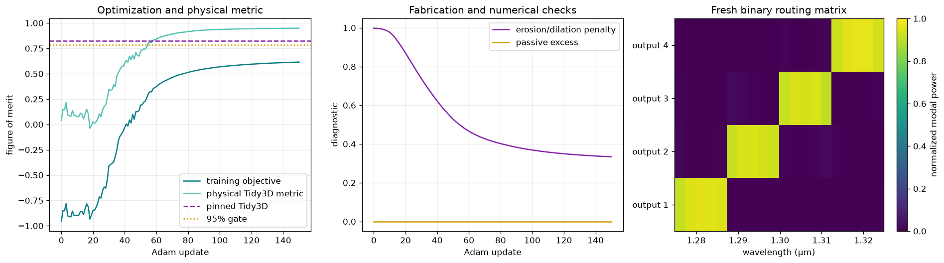
A broadband modal source and all output monitors are part of each forward solve. Reversible FDTD supplies gradients to bounded Adam while beta continuation and erosion/dilation impose the fabrication length scale. Set the flag below to repeat every adjoint. The retained notebook loads the benchmark trajectory, then always performs a fresh non-adjoint solve of its hard 0/1 material for plots and metrics.

RUN_FULL_OPTIMIZATION = False
started = perf_counter()
if RUN_FULL_OPTIMIZATION:
    result = optimize_spectral_device(CASE_ID, meta)
else:
    result = json.loads(Path("progress.json").read_text())["cases"][CASE_ID]
assert result["status"] == "pass", result
artifact = np.load(result["extras"]["best_design_artifact"], allow_pickle=True)
binary = np.asarray(artifact["binary_density"])
validation = simulate_spectral_design(CASE_ID, binary, record_fields=True)
print(f"Fresh held-out binary solve: {perf_counter() - started:.1f} s")
display(pd.DataFrame(result["metrics"]))

Fresh held-out binary solve: 46.7 s

	name	compare	got	ref	pass	error	atol	rtol	threshold
0	best_fom_parity	fom_ge	0.938132	0.784378	True	-0.153754	0.00	0.0	NaN
1	optimizer_improvement	fom_ge	1.572283	0.000100	True	-1.572183	0.00	0.0	NaN
2	passive_power_excess	scalar	0.000000	0.000000	True	0.000000	0.05	0.0	0.05
3	final_binary_fraction	fom_ge	1.000000	1.000000	True	0.000000	0.00	0.0	NaN

4. Continuous, projected, and fully binary topology

fig, axes = plt.subplots(1, 3, figsize=(15, 4.5), sharex=True, sharey=True)
design_extent = (-dx / 2, dx / 2, -dy / 2, dy / 2)
arrays = (artifact["density"], artifact["projected_density"], binary)
titles = ("Bounded optimizer parameters", "Filtered / projected state", "Fabricated 0/1 validation design")
for ax, array, title in zip(axes, arrays, titles):
    image = ax.imshow(np.asarray(array).T, origin="lower", cmap="gray_r", vmin=0, vmax=1,
                      extent=design_extent, aspect="equal", interpolation="none")
    ax.set(xlabel="x (µm)", title=title)
axes[0].set_ylabel("y (µm)")
fig.colorbar(image, ax=axes, label="core density", shrink=.78)
plt.tight_layout(); plt.show()

pd.Series({
    "binary FOM": result["extras"]["binary_fom"],
    "continuous physical FOM": result["extras"]["best_physical_fom"],
    "continuous morphology penalty": result["extras"]["best_fabrication_penalty"],
    "binary morphology penalty": result["extras"]["binary_fabrication_penalty"],
    "exact binary pixel fraction": result["extras"]["final_binary_fraction"],
}, name="value").to_frame()

	value
binary FOM	0.938132
continuous physical FOM	0.949416
continuous morphology penalty	0.333820
binary morphology penalty	0.143152
exact binary pixel fraction	1.000000

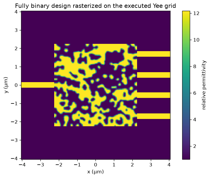
5. Actual Yee material and fresh frequency-domain fields

epsilon = validation["permittivity_xy"]
extent = validation["extent_um"]
x = np.linspace(extent[0], extent[1], epsilon.shape[0])
y = np.linspace(extent[2], extent[3], epsilon.shape[1])
fig, ax = plt.subplots(figsize=(9, 5.5))
image = ax.imshow(epsilon.T, origin="lower", extent=extent, cmap="viridis", aspect="equal")
ax.set(xlabel="x (µm)", ylabel="y (µm)", title="Fully binary design rasterized on the executed Yee grid")
fig.colorbar(image, ax=ax, label="relative permittivity"); plt.show()

fields = validation["field_intensity_xy"]
field_wavelengths = validation["field_wavelengths_um"]
fig, axes = plt.subplots(1, len(fields), figsize=(4 * len(fields), 4.2), sharex=True, sharey=True)
axes = np.atleast_1d(axes)
for ax, wavelength, intensity in zip(axes, field_wavelengths, fields):
    normalized = intensity / (intensity.max() + 1e-30)
    image = ax.imshow(normalized.T, origin="lower", extent=extent, cmap="magma", vmin=0, vmax=1, aspect="equal")
    ax.contour(x, y, epsilon.T, levels=[1.5], colors="cyan", linewidths=.35)
    ax.set(xlabel="x (µm)", title=f"λ = {wavelength:.3f} µm")
axes[0].set_ylabel("y (µm)")
fig.colorbar(image, ax=axes.tolist(), label="normalized phasor |E|²", shrink=.75)
fig.suptitle("Fresh held-out frequency-domain fields of the 0/1 design")
plt.show()

6. Convergence and spectral response

extras = result["extras"]
history = np.asarray(extras["fom_history"])
physical = np.asarray(extras["physical_fom_history"])
penalty = np.asarray(extras["fabrication_penalty_history"])
powers = np.asarray(validation["port_powers"])
wavelengths = np.asarray(spec.wavelengths_um)
fig, axes = plt.subplots(1, 3, figsize=(16, 4.5))
axes[0].plot(history, color="#087d83", label="training objective")
axes[0].plot(physical, color="#55c2b5", label="physical Tidy3D metric")
axes[0].axhline(extras["ref_fom"], color="#8221a8", ls="--", label="pinned Tidy3D")
axes[0].axhline(extras["threshold"], color="#d29b00", ls=":", label="95% gate")
axes[0].set(xlabel="Adam update", ylabel="figure of merit", title="Optimization and physical metric")
axes[0].legend(); axes[0].grid(alpha=0.25)

axes[1].plot(penalty, color="#8221a8", label="erosion/dilation penalty")
axes[1].plot(np.asarray(extras["passive_excess_history"]), color="#d29b00", label="passive excess")
axes[1].set(xlabel="Adam update", ylabel="diagnostic", title="Fabrication and numerical checks")
axes[1].legend(); axes[1].grid(alpha=.25)

if spec.objective == "wdm":
    response = axes[2].imshow(powers, origin="lower", cmap="viridis", vmin=0, vmax=1,
                              extent=(wavelengths[0], wavelengths[-1], -0.5, powers.shape[0] - 0.5), aspect="auto")
    axes[2].set_yticks(range(powers.shape[0]), [f"output {index + 1}" for index in range(powers.shape[0])])
    axes[2].set(xlabel="wavelength (µm)", title="Fresh binary routing matrix")
    fig.colorbar(response, ax=axes[2], label="normalized modal power")
else:
    axes[2].plot(wavelengths, powers[0], "o-", color="#087d83")
    axes[2].axvspan(0.91, 1.01, color="#55c2b5", alpha=0.25, label="passband")
    axes[2].set(xlabel="wavelength (µm)", ylabel="normalized modal power", title="Fresh binary transmission")
    axes[2].legend(); axes[2].grid(alpha=0.25)
plt.tight_layout(); plt.show()

pd.Series({
    "best FDTDX FOM": extras["best_fom"],
    "pinned Tidy3D FOM": extras["ref_fom"],
    "required threshold": extras["threshold"],
    "actual updates": extras["iterations_run"],
    "best update": extras["best_iteration"],
    "projection beta": extras["best_beta"],
}, name="value").to_frame()

	value
best FDTDX FOM	0.938132
pinned Tidy3D FOM	0.825661
required threshold	0.784378
actual updates	150.000000
best update	150.000000
projection beta	50.000000

Reproduce and refine

These retained plots are executed locally, not copied from the golden. The reported FOM comes from the fully binary, fixed-threshold geometry and an independent non-differentiable solve. The projected gray state is shown only to make the optimization mechanics auditable. Production sign-off should additionally refine the Yee mesh and evaluate erosion/dilation process corners.

print("uv run fdtdx-bench run --case invdes_wdm")

uv run fdtdx-bench run --case invdes_wdm