Modal-current temporal cavity campaign

Live optimizer

This fresh campaign replaces the point dipole and point sample by a fixed feedthrough-mode current sheet and its reciprocal modal coordinate. From the first solve it minimizes error to one fixed, unity-amplitude causal lossless waveform. No amplitude or phase is fitted per step.

State	Value
Status	running_shifted_lossless_temporal_level_set
Source	fixed_feedthrough_mode_electric_current
Temporal observable	fixed_scale_reciprocal_mode_electric_coordinate
Phase	shifted_lossless_temporal_level_set
Active coordinates	subpixel_level_set_boundary
Completed updates	72
Temporal objective	-0.9737
Whole-trace fixed-waveform fidelity	0.50666
Source-off fixed-waveform fidelity	0.5062
Fixed target source-off power (telemetry)	0.50004
Fixed-target gain (ideal = 1)	0.013273
Fixed-target normalized MSE	0.9737
Normalized temporal residual	0.98676
Full-field coherence	0.99999
Shifted stationarity	0.80338
Q telemetry	560.07
Normalized V telemetry	0.059597
Active pole tape	1 ps
Maxwell-step reduction vs 2 ps	2×
Projection stage	modal_binary_mature
Projection beta / eta	48 / 0.50
Gray fraction	2.28%
Material optimizer	adaptive_trust_region_lbfgsb_v1
Material coordinates	smooth spline phase field; no density pixels
Material trust radius	0.00562 µm
L-BFGS memory pairs	0
Forward-only rejected-step retries	561
Boundary handoff	replay_passed_level_set_active
Stable binary-topology states	1 / 1
Boundary trust radius	5e-05 µm
Last candidate accepted	False
Last pole trustworthy	True
Latest update wall time	4.089 s
Last artifact write	2026-08-28 23:09:12 UTC

The authoritative state is benchmarks/artifacts/invdes_fryett_modal_temporal_modal_current_v4_4d_beta.npz. The stopped point-source temporal checkpoint is a separate preserved artifact; this modal campaign did not seed from or otherwise modify it.

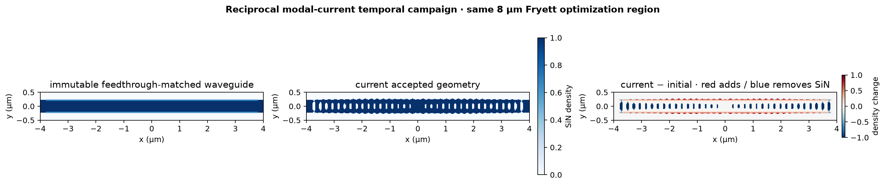
Geometry and exact material difference

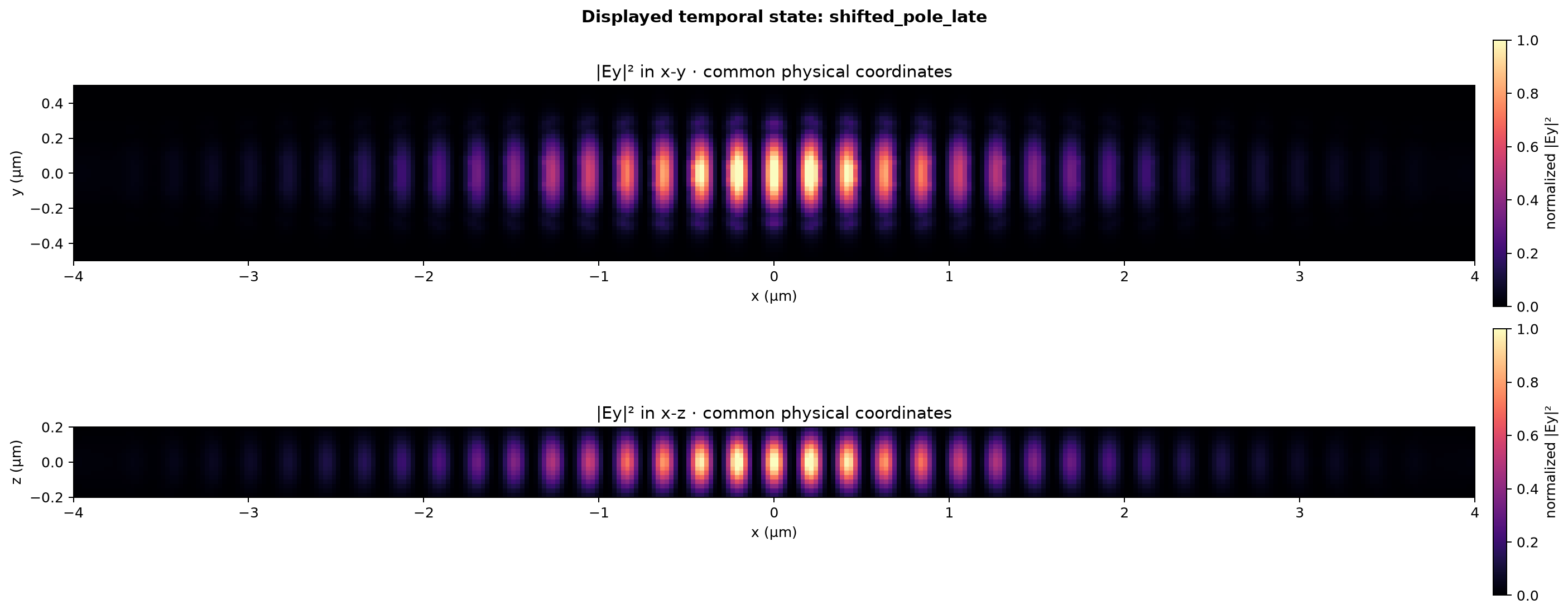
Field used by the temporal objective

Exact temporal target response

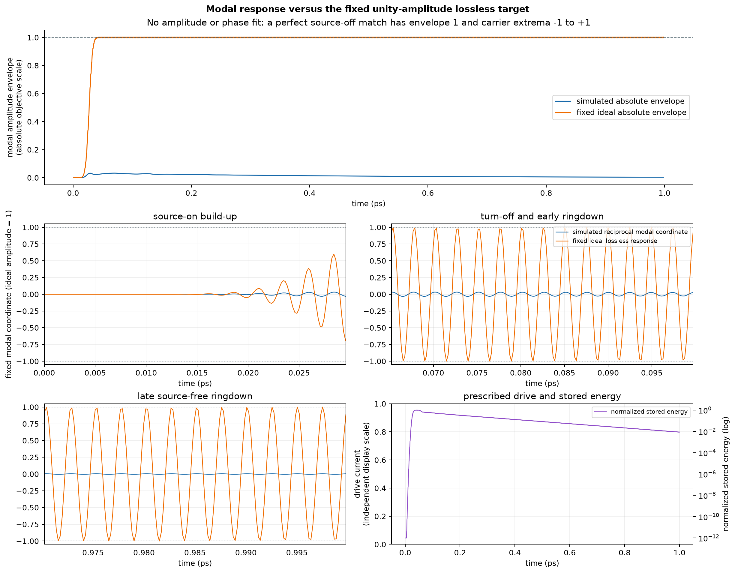
The orange curve is the fixed causal convolution of the prescribed current waveform with the cosine Green function of one lossless pole. It is not the source waveform and is not fitted to the simulation. During the drive it contains the exact causal build-up; after turn-off its extrema are exactly -1 and +1. The blue simulation is plotted in those same absolute objective units, so a smaller blue envelope is a real amplitude error, not a display normalization. The current waveform appears only in the diagnostic panel on its own explicitly independent display scale. The former blue background bands were 4D field-snapshot windows; they were never objective weights and have been removed from this plot to make the absolute comparison unambiguous. Every temporal sample still enters the single normalized mean-square error equally.

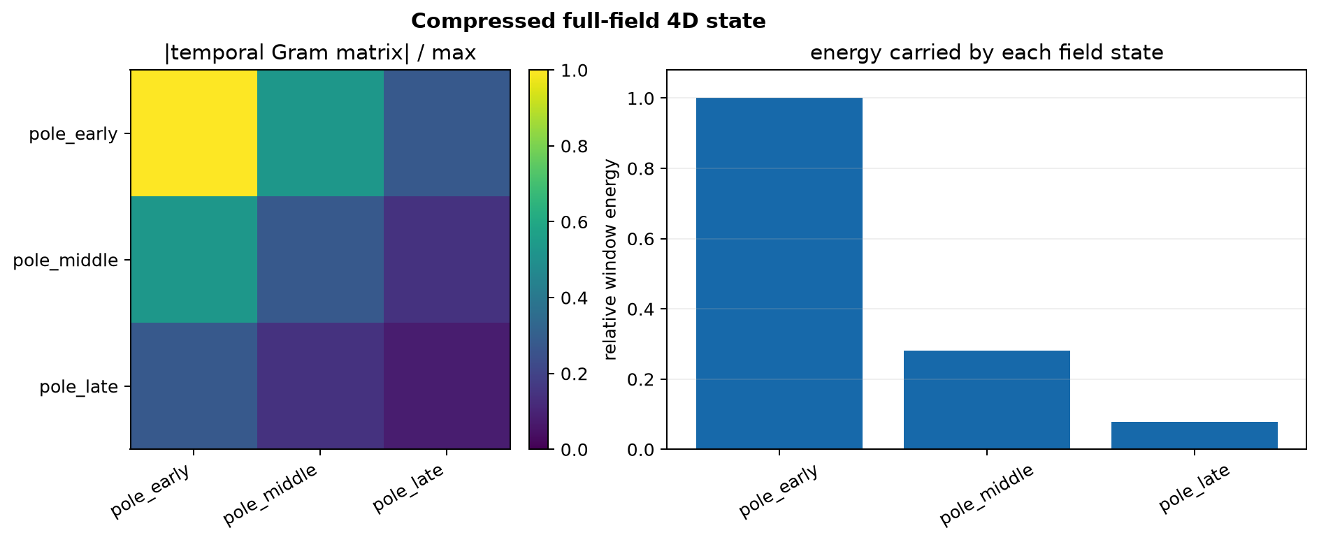
Full-field temporal correlations

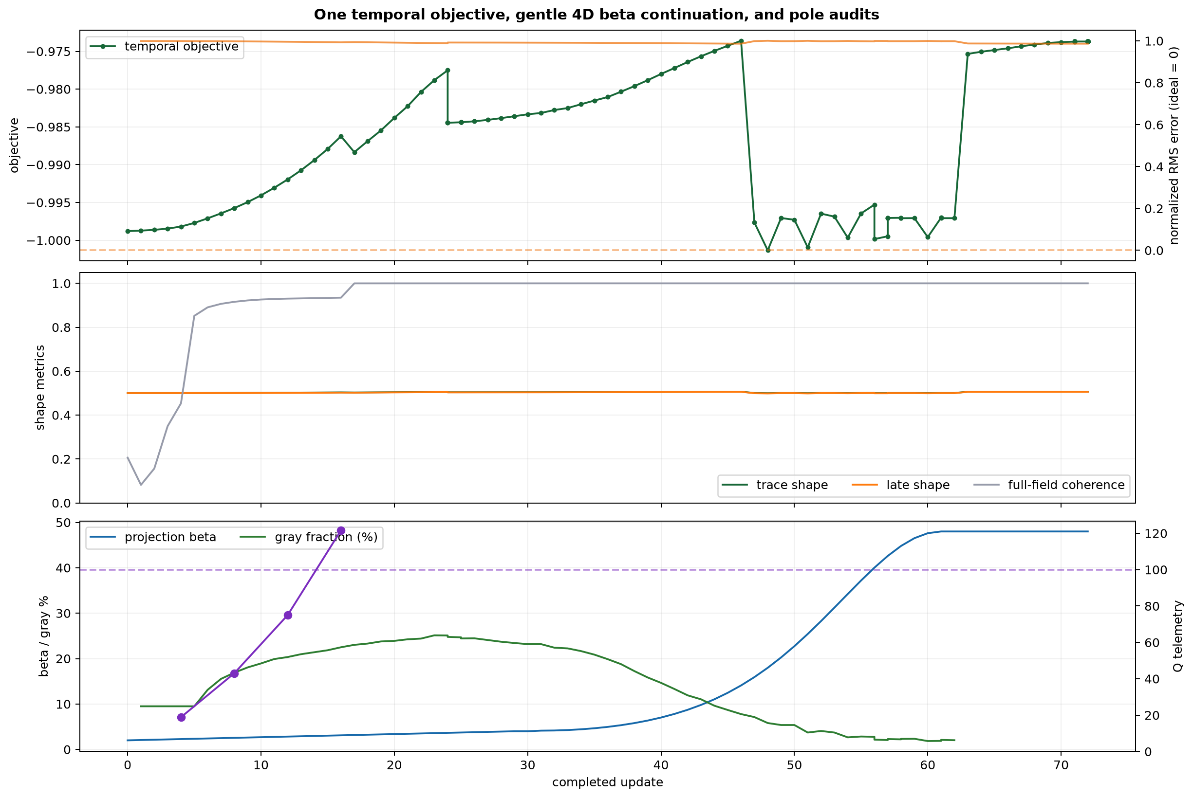
Objective, binarization, and pole history

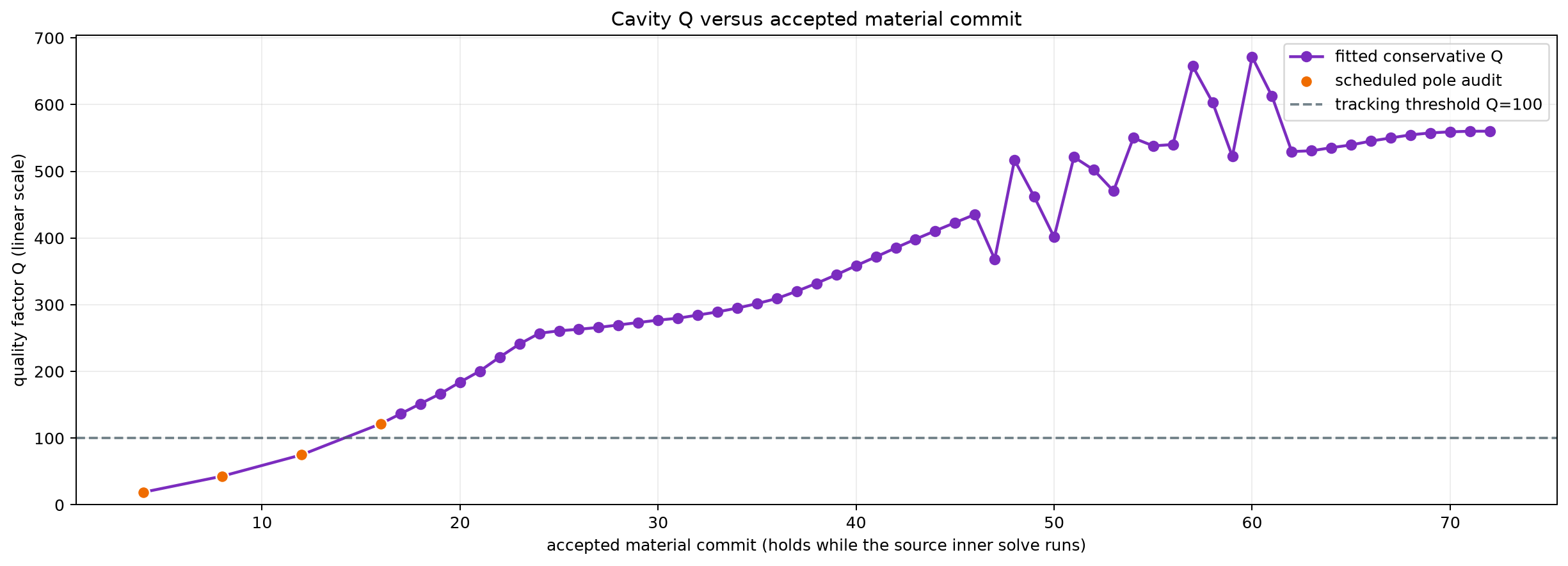
Q versus accepted material commit — linear scale

Modal-current fixed-waveform cavity campaign

Purpose

This campaign tests a deliberately literal inverse-design objective: make the complete observed time trace equal the response of one perfectly mapped, lossless cavity mode. It replaces both the three-dimensional point dipole and the point sample by a reciprocal distributed waveguide-mode current and modal coordinate, forming a reciprocal, distributed source/observable pair. The optimization region remains the same 8 µm × 1 µm Fryett region. There is no DCT preconditioner, lattice, mirror period, radial weighting, output-mode term, mode-volume term, late-time-power term, or field-correlation term is imposed.

The hypothesis is that a point source encourages a local antenna because its three-dimensional Green function strongly weights nearby material. An ideal one-dimensional guided Green function instead has approximately constant longitudinal magnitude,

[ G_{1\mathrm D}(x,x_0;\omega) = \frac{i}{2v_g}e^{i\beta|x-x_0|}, \qquad |G_{1\mathrm D}|\simeq\frac{1}{2v_g}. ]

Remote pixels must still cooperate through phase, but they are not suppressed by a point-source near field. This does not force periodicity; it is a test of whether the collective source and exact temporal target are sufficient.

The initial material field is a continuous 450 nm-wide SiN waveguide across the full 8 µm design length, exactly matching the terminal feedthrough width. In the symmetry-reduced half-width domain this occupies cell centers (0\le y<225) nm. The ordinary fabrication filter and beta-2 projection give its edge the same differentiable subpixel transition used by every later candidate. This is an initialization, not a frozen geometry: every interior pixel, including the source plane, remains trainable; only the final 200 nm terminal feedthrough cells are pinned.

Fixed modal current and reciprocal coordinate

At the target frequency (f_0=c/(780,\mathrm{nm})), the mode solver computes the fundamental TE mode of the terminal 450 nm-wide, 250 nm-thick SiN feedthrough. Let its phase-fixed electric profile be (\mathbf e_s(y,z)). The impressed current is

[ \mathbf J(\mathbf r,t) =J_0\mathbf e_s(y,z)\delta(x)s(t), ]

where (s(t)) is the broadband Gaussian pulse. It is an electric-only soft current sheet, so it radiates in both longitudinal directions. In the symmetry-reduced simulation its first-cell deposit has the exact half weight needed to preserve the unfolded current moment.

The observed scalar is the matching electric modal coordinate

[ q(t)=\sum_A \mathbf e_d(y,z)\cdot\mathbf E(x=0,y,z,t)w_A. ]

The source and detector use the same Yee-component locations and face weights; detector interpolation is disabled for this coordinate. Consequently the forward current and adjoint observation are a reciprocal distributed pair. The temporary terminal-guide material sheet is used only while the two fixed profiles are cached. Every physical run overwrites the complete trainable plane with the candidate density, so no central waveguide shape is forced.

Exact causal lossless target

An electric-current impulse changes the electric modal coordinate directly. The discrete ideal response is therefore a causal cosine convolution, not a free sine/cosine fit. At the full FDTD cadence, define

[ \theta_n=2\pi f n\Delta t,\qquad C_n=\sum_{m\le n}s_m\cos\theta_m,\qquad S_n=\sum_{m\le n}s_m\sin\theta_m, ]

[ g_n=\cos\theta_n C_n+\sin\theta_n S_n =\sum_{m\le n}s_m\cos[2\pi f(n-m)\Delta t]. ]

This includes the pulse-on transient. After the pulse, (C_n) and (S_n) are constant and (g_n) is exactly one nondecaying sinusoid at (f).

The amplitude scale is also fixed analytically. If (\mathbf e_s) is the current profile, (\mathbf e_d) the detector profile, and (\epsilon_{\rm ref}^{-1}) the inverse permittivity against which the profiles were cached, the one-step discrete coupling is

[ \kappa=C_{\rm CFL}a_s a_c \sum_A \mathbf e_d\cdot (\epsilon_{\rm ref}^{-1}\mathbf e_s)w_A, ]

where (a_s) contains the fixed source amplitudes and (a_c=1/2) is the centered symmetry-plane weight. Let

[ A_s=\sqrt{C_N^2+S_N^2},\qquad y_n^*=-\frac{\kappa g_n}{|\kappa|A_s},\qquad y_n=\frac{q_n}{|\kappa|A_s}. ]

Thus the ideal source-off oscillation has amplitude one. Unity is a reporting convention, but the map from the raw simulated coordinate to unity is fixed by the discrete source/detector coupling. It is not recomputed from (q_n), and neither amplitude nor phase is fitted at any optimization step. A zero trace, a half-amplitude trace, and a double-amplitude trace all have nonzero error. The raw modal trace is not DC-subtracted because DC is part of the specified waveform error.

The sole scalar objective is

[ F(\rho)=-\frac{\sum_n[y_n(\rho)-y_n^]^2} {\sum_n(y_n^)^2}. ]

There is no separate late-time-power reward and no coherence, stationarity, pole-fit, Q, V, or Q/V term in (F). The dashboard reports the normalized RMS error, the fixed-target gain (\langle y,y^\rangle/\langle y^,y^*\rangle), and two bounded waveform fidelities, but none is used to rescale the target.

Pole tracking and minimum viable tape

Every fourth pixel update performs a diagnostic pole audit. Once a trustworthy pole has (Q\ge100), its real frequency becomes the carrier and target frequency for the next turn. Within an acceptance comparison, incumbent and candidate always use the same frozen frequency; a candidate’s fitted pole cannot move its own target. Pole estimates, fit residuals, Q, and the 4D field states remain telemetry and safety gates only.

The ringdown tape is the shortest compiled tier in ({0.40,0.65,1.00,1.50,2.00}) ps that contains at least 1.5 fitted field-amplitude lifetimes plus the analysis margin. Increasing the tape changes only how long the same fixed-waveform MSE is evaluated.

Pixel steps use adaptive trust-region L-BFGS-B with eight accepted secant pairs. The L-BFGS direction is projected into the material box and the fixed terminal cells, then truncated to an infinity-norm latent trust radius. There is no Q-dependent density-motion cap and no DCT or radial conditioning.

One differentiated incumbent evaluation supplies the objective and gradient. The candidate costs one forward solve. With

[ p_k=\nabla F_k^T\Delta\rho_k,\qquad r_k=\frac{F(\rho_k+\Delta\rho_k)-F(\rho_k)}{p_k}, ]

the trial is accepted only when its objective rises and (r_k\ge0.05). A rejection halves the trust radius. Agreement (r_k\ge0.75) expands it by 1.5 when at least 80% of the radius was used. Crucially, a rejection does not advance beta, move the carrier, or recompute the adjoint: the incumbent gradient is persisted and the smaller retry costs one forward solve. After three consecutive rejections the stale curvature pairs are cleared, but the same cached gradient is retained. Beta increments do not clear L-BFGS memory.

Gentle 4D-Q/V beta continuation and smooth-boundary handoff

This campaign reuses the beta curve from the 4D Q/V campaign, indexed by accepted geometry updates. For (0\le k<30),

[ \beta_k=2+\frac{2k}{29}. ]

Update 30 holds beta at 4. For (31\le k\le61), let

[ t=(k-31)/30,\qquad s(t)=t^2(3-2t), ]

[ \beta_k=\exp!\left[\log(4+8/59) +s(t)\log!\frac{48}{4+8/59}\right]. ]

Beta then remains 48. Once beta reaches 12, the projection threshold cycles through (\eta=0.50,0.47,0.53), as in the 4D campaign, so a purported binary topology must survive nearby thresholds. Rejected trust trials do not advance this schedule because they reuse the incumbent gradient; this preserves the one-adjoint-per-location rule. Beta or eta changes do not reset L-BFGS memory.

Hard thresholding is not used inside the pixel-gradient loop because its derivative is zero. Once beta is 48 and at most 4% of cells lie between 0.1 and 0.9, the density is thresholded at 0.5 to define an exact binary topology. A subpixel level set is fitted to that topology and replayed through Maxwell. Only physical interface cells are gray after this point; they represent subpixel area averaging of a sharp boundary, not a mixed material design.

One eligible binary state triggers the replay attempt. It fails closed unless the topology is preserved, the fixed-waveform fidelity is retained, the field state overlaps the pixel incumbent, and the pole remains trustworthy. The same fixed waveform MSE then moves only the topology-safe level-set boundary using adaptive trust-region L-BFGS. A level set is used instead of free splines because it already supports multiple components, subpixel averaging, exact topology checks, and local normal motion without prescribing how many holes the cavity must contain.

Moving and fixed components

Fixed throughout:

• 8 µm × 1 µm optimization region, 25 nm grid, stack, symmetry, and PML;

• fixed feedthrough TE source and reciprocal detector profiles;

• analytic source/detector amplitude calibration;

• one causal lossless waveform and one normalized-MSE objective;

• the eta policy: 0.50 below beta 12, then the 0.50/0.47/0.53 robustness cycle;

• no periodicity, DCT, output coupling, mode-volume, or late-power objective.

Moving during pixels:

• all trainable raw pixels, including the source plane;

• projection beta according to the accepted-step 4D Q/V continuation;

• the adaptive latent trust radius, with no Q-dependent density cap;

• after trustworthy Q≥100, the common next-turn carrier and tape tier.

Moving after handoff:

• only the subpixel level-set boundary in its narrow band;

• the adaptive topology-safe boundary trust radius and occasional exact chart rebase (which clears coordinate-specific L-BFGS memory);

• the same tracked carrier and tape controller;

• never the target amplitude or per-turn phase.

Prepared state and launch policy

Initialization creates a distinct v4 4D-beta trust-L-BFGS artifact from the continuous feedthrough-matched guide and a dashboard in ready_not_started state. It does not run Maxwell or start a service. The v1 free-amplitude modal artifact and the stopped point-source checkpoint remain preserved as separate artifacts.

Operations

A bounded manual turn can be run with:

FDTDX_FRYETT_MODAL_TEMPORAL_ID=modal_current_v4_4d_beta uv run python -m benchmarks.cases.invdes_fryett_hybrid_scratch.modal_temporal --updates 1

The persistent launcher is scripts/start_fryett_modal_temporal_campaign.sh.