Nanobeam cavity: resonant wavelength and quality factor

This notebook reconstructs the tapered-hole silicon nanobeam from the official Tidy3D NanobeamCavity.ipynb example and executes it locally with FDTDX. It follows the full workflow: define physical parameters, construct and inspect the geometry, run the time-domain simulation, plot the recorded electric field and ringdown, and extract the resonant wavelength and \(Q\) with harmonic inversion.

The compact benchmark retains the published cubic lattice/radius taper, a 500 nm × 220 nm silicon beam, four constant mirror cells per side, eight tapered cells, a broadband \(E_y\) dipole, mirror symmetry, and a 3 ps ringdown. The final comparison uses the same pole extractor for FDTDX and the frozen Tidy3D signal.

Imports and accelerator

import os
os.environ.setdefault("XLA_PYTHON_CLIENT_PREALLOCATE", "false")

from time import perf_counter
import warnings
import matplotlib.pyplot as plt
from matplotlib.patches import Circle, Rectangle
import numpy as np
import pandas as pd
import jax
import fdtdx
from IPython import get_ipython

from benchmarks.cases.device_nanobeam_cavity.run import (
    NanobeamParameters,
    _dominant_resonance,
    build_nanobeam_simulation,
)
from benchmarks.device_geometry import nanobeam_holes_um

get_ipython().run_line_magic("matplotlib", "inline")
warnings.filterwarnings("ignore", category=FutureWarning, module=r"tidy3d\.components\.mode")
plt.rcParams.update({"figure.figsize": (9, 4.5), "figure.dpi": 120})
print(f"FDTDX {fdtdx.__version__ if hasattr(fdtdx, '__version__') else 'local'}")
print(f"JAX devices: {jax.devices()}")

FDTDX local
JAX devices: [CudaDevice(id=0)]

1. Physical and numerical parameters

Lengths are entered in micrometres for readability. NanobeamParameters is an immutable input record; changing a field and rebuilding the scene is enough to run a resolution, runtime, or geometry study.

parameters = NanobeamParameters(
    grid_spacing_um=0.025,
    run_time_ps=3.0,
    wavelength_window_um=(1.4, 1.6),
    beam_width_um=0.500,
    beam_thickness_um=0.220,
    silicon_index=3.5,
    oxide_index=1.44,
    pml_layers=12,
)
pd.Series(parameters._asdict(), name="value").to_frame()

	value
grid_spacing_um	0.025
interior_um	(8.4, 3.7, 3.4)
run_time_ps	3.0
analysis_start_ps	0.2
wavelength_window_um	(1.4, 1.6)
pml_layers	12
beam_width_um	0.5
beam_thickness_um	0.22
silicon_index	3.5
oxide_index	1.44

2. Geometry construction

The hole centers and radii below are the arrays used to instantiate the FDTDX cylinders—not a separate illustration. The lattice constant and hole radius taper cubically toward the central defect.

centers_um, radii_um = nanobeam_holes_um()

fig, ax = plt.subplots(figsize=(12, 2.8))
ax.add_patch(Rectangle(
    (-parameters.interior_um[0] / 2, -parameters.beam_width_um / 2),
    parameters.interior_um[0], parameters.beam_width_um,
    facecolor="#55c2b5", edgecolor="#087d83", label="silicon beam",
))
for center, radius in zip(centers_um, radii_um, strict=True):
    ax.add_patch(Circle((center, 0), radius, facecolor="white", edgecolor="#18364a"))
ax.set(
    xlim=(-4.3, 4.3), ylim=(-0.55, 0.55), aspect="equal",
    xlabel="x (µm)", ylabel="y (µm)", title="Exact tapered-hole geometry",
)
ax.legend(loc="upper right")
plt.show()

pd.DataFrame({"x_center_um": centers_um, "radius_um": radii_um}).head(8)

	x_center_um	radius_um
0	-2.975000	0.120400
1	-2.545000	0.120400
2	-2.115000	0.120400
3	-1.685000	0.120400
4	-1.262812	0.116025
5	-0.865625	0.106400
6	-0.502812	0.096775
7	-0.165000	0.092400

3. Build and voxelize the FDTDX scene

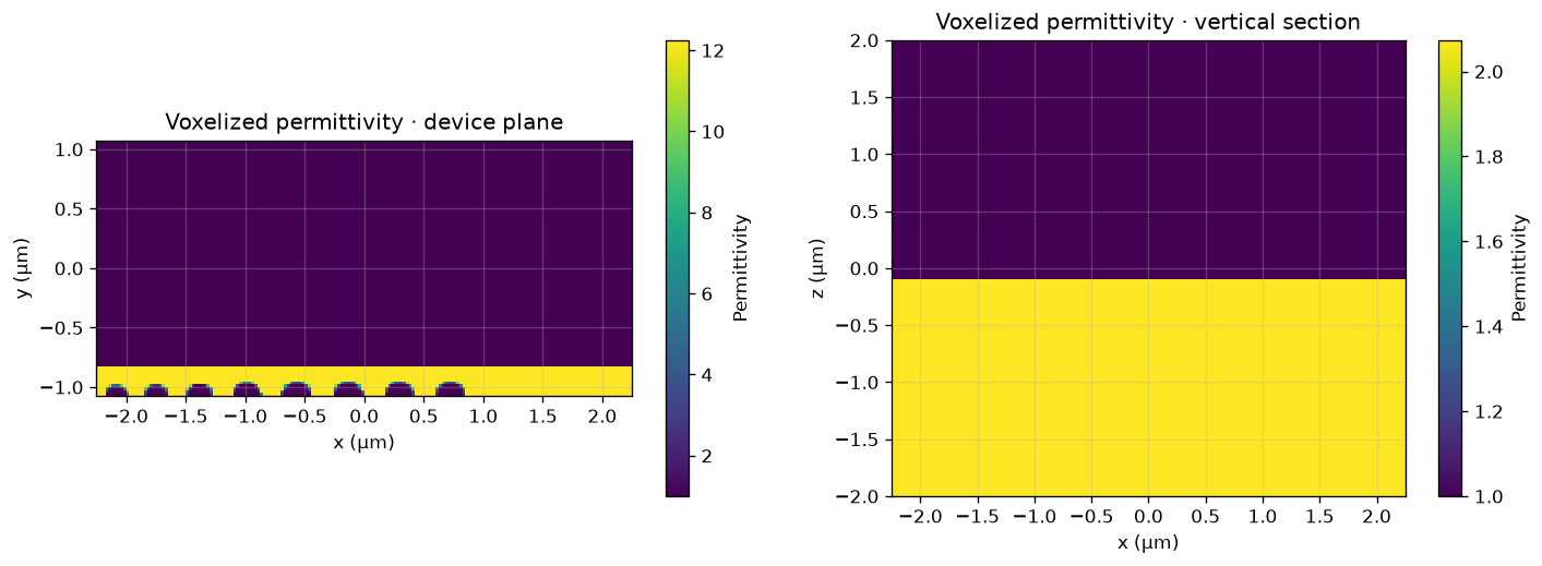
The builder creates the simulation volume, oxide substrate, silicon beam, air-hole cylinders, broadband dipole, ringdown monitor, PML, uniform grid, and mirror planes. Placement and parameter application produce the arrays that the solver will actually update.

object_list, constraints, config = build_nanobeam_simulation(parameters)
key = jax.random.PRNGKey(0)
objects, arrays, design_params, config, placement_info = fdtdx.place_objects(
    object_list=object_list,
    config=config,
    constraints=constraints,
    key=key,
)
arrays, objects, _ = fdtdx.apply_params(arrays, objects, design_params, key)

print(f"Reduced Yee grid: {objects.volume.grid_shape}")
print(f"Time steps: {config.time_steps_total:,}")
print(f"Δt: {config.time_step_duration * 1e18:.3f} as")
print(f"Objects: {len(objects.object_list)}")

Reduced Yee grid: (180, 86, 160)
Time steps: 62,940
Δt: 47.664 as
Objects: 18

fig, axes = plt.subplots(1, 2, figsize=(12, 4.2))
fdtdx.plot_material_from_side(
    config, arrays, viewing_side="z", position=0.0,
    material_axis=0, plot_legend=True, ax=axes[0],
)
fdtdx.plot_material_from_side(
    config, arrays, viewing_side="y", position=0.0,
    material_axis=0, plot_legend=True, ax=axes[1],
)
axes[0].set_title("Voxelized permittivity · device plane")
axes[1].set_title("Voxelized permittivity · vertical section")
plt.tight_layout()
plt.show()

4. Run the simulation

run_fdtd advances the same placed arrays used by the benchmark. No Tidy3D service or cached field data is involved. The broadband dipole switches off early; the high-Q mode remains and is sampled every second time step by the point monitor.

started = perf_counter()
_, result_arrays = fdtdx.run_fdtd(
    arrays=arrays,
    objects=objects,
    config=config,
    key=key,
    show_progress=False,
)
elapsed_s = perf_counter() - started
print(f"Local FDTDX runtime: {elapsed_s:.1f} s")

Local FDTDX runtime: 29.6 s

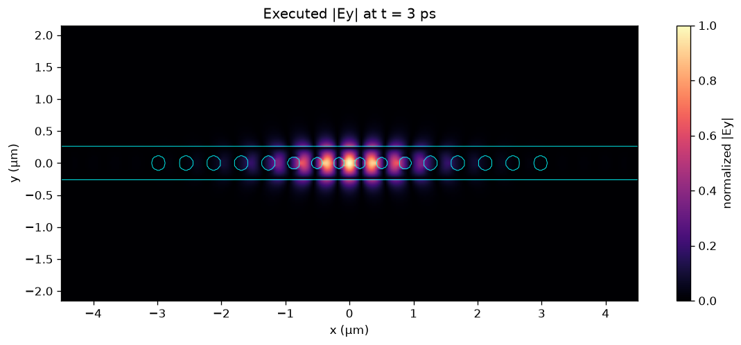
5. Plot the simulated cavity field

# The final full-domain field is still finite because the cavity rings down slowly.
ey_reduced = np.asarray(result_arrays.fields.E[1])
ey_xy = ey_reduced[:, :, ey_reduced.shape[2] // 2]
eps_reduced = 1 / np.asarray(result_arrays.inv_permittivities[1])
eps_xy = eps_reduced[:, :, eps_reduced.shape[2] // 2]

# Reconstruct the magnitude on both mirror-reduced axes for display.
ey_abs = np.abs(ey_xy)
ey_full = np.concatenate((ey_abs[::-1], ey_abs), axis=0)
ey_full = np.concatenate((ey_full[:, ::-1], ey_full), axis=1)
eps_full = np.concatenate((eps_xy[::-1], eps_xy), axis=0)
eps_full = np.concatenate((eps_full[:, ::-1], eps_full), axis=1)

extent = [
    -parameters.interior_um[0] / 2 - parameters.pml_layers * parameters.grid_spacing_um,
    parameters.interior_um[0] / 2 + parameters.pml_layers * parameters.grid_spacing_um,
    -parameters.interior_um[1] / 2 - parameters.pml_layers * parameters.grid_spacing_um,
    parameters.interior_um[1] / 2 + parameters.pml_layers * parameters.grid_spacing_um,
]
fig, ax = plt.subplots(figsize=(12, 4.3))
image = ax.imshow(
    ey_full.T / (ey_full.max() + 1e-30), origin="lower", extent=extent,
    cmap="magma", vmin=0, vmax=1, aspect="equal",
)
ax.contour(
    np.linspace(extent[0], extent[1], eps_full.shape[0]),
    np.linspace(extent[2], extent[3], eps_full.shape[1]),
    eps_full.T, levels=[2.0], colors="cyan", linewidths=0.55,
)
ax.set(xlabel="x (µm)", ylabel="y (µm)", title="Executed |Ey| at t = 3 ps")
fig.colorbar(image, ax=ax, label="normalized |Ey|")
plt.show()

6. Ringdown and harmonic-inversion analysis

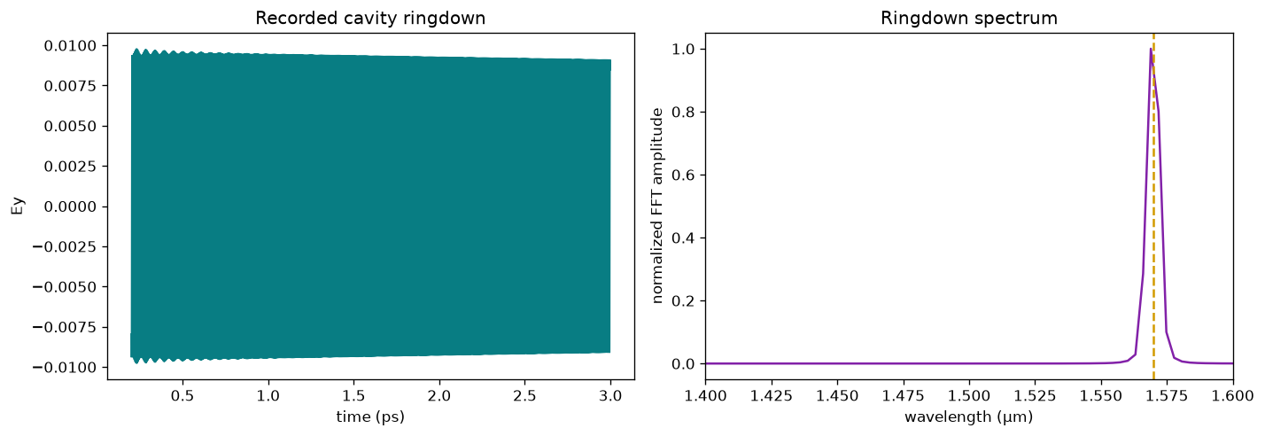
A Fourier peak alone cannot reliably determine a \(Q\) near \(3 imes10^4\) from this compact time window. The same ResonanceFinder pole extraction is therefore applied to both the FDTDX signal and the frozen Tidy3D signal used by the benchmark.

signal = np.asarray(result_arrays.detector_states["ringdown"]["fields"][:, 0])
sample_dt = 2 * config.time_step_duration
time_ps = parameters.analysis_start_ps + np.arange(signal.size) * sample_dt * 1e12
resonance = _dominant_resonance(signal, sample_dt)

fig, axes = plt.subplots(1, 2, figsize=(12, 4.2))
axes[0].plot(time_ps, signal, lw=0.7, color="#087d83")
axes[0].set(xlabel="time (ps)", ylabel="Ey", title="Recorded cavity ringdown")

frequencies = np.fft.rfftfreq(signal.size, sample_dt)
spectrum = np.abs(np.fft.rfft(signal * np.hanning(signal.size)))
wavelength_um = fdtdx.constants.c / frequencies[1:] * 1e6
axes[1].plot(wavelength_um, spectrum[1:] / spectrum[1:].max(), color="#8221a8")
axes[1].axvline(resonance["wavelength_um"], color="#d29b00", ls="--")
axes[1].set(
    xlim=parameters.wavelength_window_um, xlabel="wavelength (µm)",
    ylabel="normalized FFT amplitude", title="Ringdown spectrum",
)
plt.tight_layout()
plt.show()

pd.DataFrame(resonance["candidates"])

	wavelength_um	Q	amplitude	error
0	1.56993	31370.13106	0.004802	0.000016

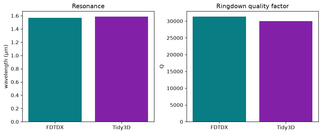
7. Compare wavelength and Q with the pinned Tidy3D result

golden = np.load("benchmarks/goldens/device_nanobeam_cavity.npz", allow_pickle=True)
comparison = pd.DataFrame(
    {
        "FDTDX": [resonance["wavelength_um"], resonance["Q"]],
        "Tidy3D": [float(golden["wavelength_um"][0]), float(golden["Q"][0])],
    },
    index=["resonant wavelength (µm)", "quality factor Q"],
)
display(comparison)

fig, axes = plt.subplots(1, 2, figsize=(9, 3.8))
axes[0].bar(comparison.columns, comparison.loc["resonant wavelength (µm)"], color=["#087d83", "#8221a8"])
axes[0].set(ylabel="wavelength (µm)", title="Resonance")
axes[1].bar(comparison.columns, comparison.loc["quality factor Q"], color=["#087d83", "#8221a8"])
axes[1].set(ylabel="Q", title="Ringdown quality factor")
plt.tight_layout()
plt.show()

	FDTDX	Tidy3D
resonant wavelength (µm)	1.56993	1.588007
quality factor Q	31370.13106	29979.880637

Result and next checks

This notebook establishes the scoped benchmark: a locally executed FDTDX cavity field, a reliable pole in the requested wavelength window, and wavelength/Q agreement within the declared case tolerances. For a publication result, repeat at finer spatial resolution, lengthen the ringdown, vary the fitting window, and verify convergence of every reported pole rather than relying on this compact parity configuration.